[DSP] W01 - Basics

• obligatory dead person quote:
  • ”[…] space and time are mere thought entities and creatures of the imagination […] They precede the existence of objects of the senses […]”
• number sets:
  • $N$: natural numbers $[1,\infty )$
    • whole numbers $[0,\infty )$
  • $Z$: integers
  • $Q$: rational numbers
    • inclusive of recurring mantissa
  • $P$: irrational numbers
    • non-repeating and non-recurring mantissa
    • $\pi$ value, $\sqrt{2}$
  • $R$: real numbers (everything on the number line)
    • includes rational and irrational numbers
  • $C$: complex numbers
    • includes real and imaginary numbers

fig: number sets

---

digital signal processing

• signal: description of a physical phenomenon’s evolution over time
• signal processing:
  • analysis: understanding the information carried by the signal
  • synthesis: creating a signal to contain the information
• digital paradigm for signal processing:
  • discrete, digitized time
  • discrete, digitized amplitude
• a digital signal is a sequence of observations called samples
  • a sample is denoted by $x\left[n\right]$
• each sample is subjected to both:
  • time discretization: time component ‘$n$’
  • amplitude discretization: amplitude component ‘$x$’

discrete-time

• discrete-time model:
  • a paradigm that moves away from the idealistic analog view
    • makes computation more intuitive
    • finding solutions easier with computational methods
  • more practical model of reality compared to analog models
• Sampling Theorem:
  • mathematically, analog and discrete models are equivalent
    • provided sufficient discrete sampling is available
• samples replace idealized models
• simple math replaces calculus

discrete-amplitude

• each amplitude can only take on a value from a predetermined set
  • the number of levels in countable
  • so the amplitude is mapped to a set of integers
• this ability to integer mapping provides benefits for
  • storage
  • processing
  • transmission
• analog signals suffer from noise and attenuation in way that causes loss of information during signal transmission
  • digital signal transmission mechanisms are more robust
  • information is significantly low
• general-purpose storage can be used
• general-purpose processing can be applied
• noise can be controlled during signal transmission

---

discrete-time signals

• ‘lollipop’ notation
• discrete-time signals sampled sufficiently densely look continuous in a plot

formally

• a sequence of complex numbers
• one dimensional
• notation: $x\left[n\right]$
  • $\left[n\right]$: integer
• two-sided sequences: $x:Z\to C$
  • $n\in (-\infty ,+\infty )$
• $n$ is adimensional “time”
  • no physical units, just a counter
  • can embody periodicity
    • number of samples of the repeating pattern
• analysis eg.: periodic temperature, sea-level, river water level
• synthesis eg.: stream of algorithm generated samples

fundamental discrete signals

• delta signal: $x\left[n\right]=\delta \left[n\right]$
  • when $n=0,x=1$; else $x=0$
  • signifies a physical phenomenon that lasts a very short duration of time
  • eg. a clapper for syncing video and audio for a movie recording
    • when audio and video recording happens separately

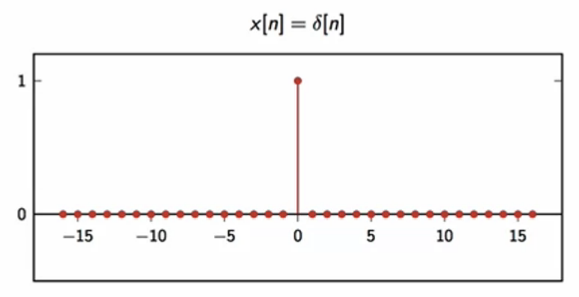
fig: discrete delta

• unit step: $x\left[n\right]=u\left[n\right]$
  • when $n<0,x=0$; else $x=1$
  • synonymous to flipping a switch

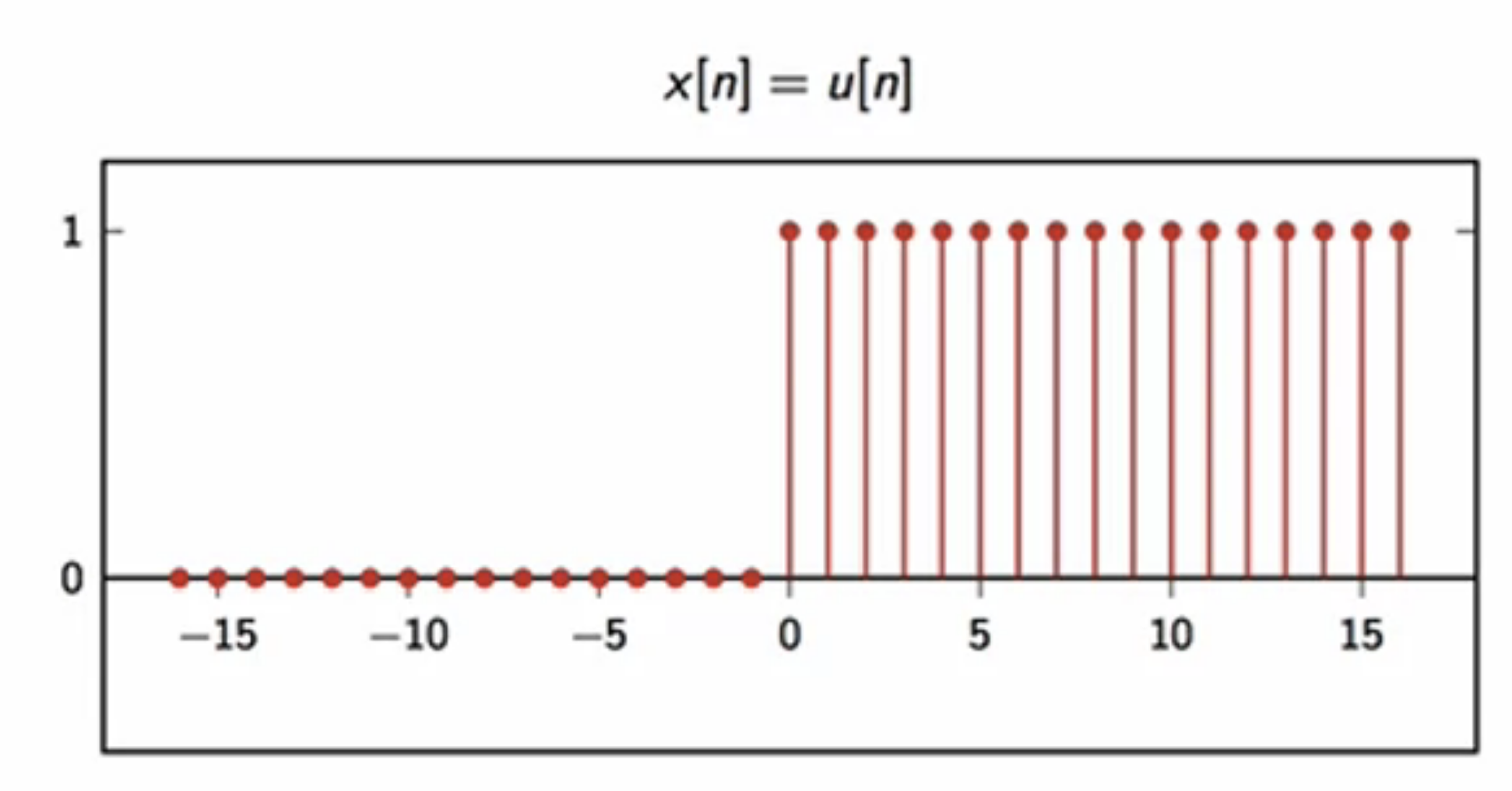
fig: discrete unit step

• exponential decay: $x\left[n\right]=\left|a{|}^{n}u\right[n],|a|<1$
  • when $n<0,x=0$; else $x$ decays exponentially, starting from $1$ @ $n=0$
  • $x\to 0$ as $n\to \infty$
  • newton’s law of cooling
    • cooling of a coffee cup
  • rate of capacitor discharge

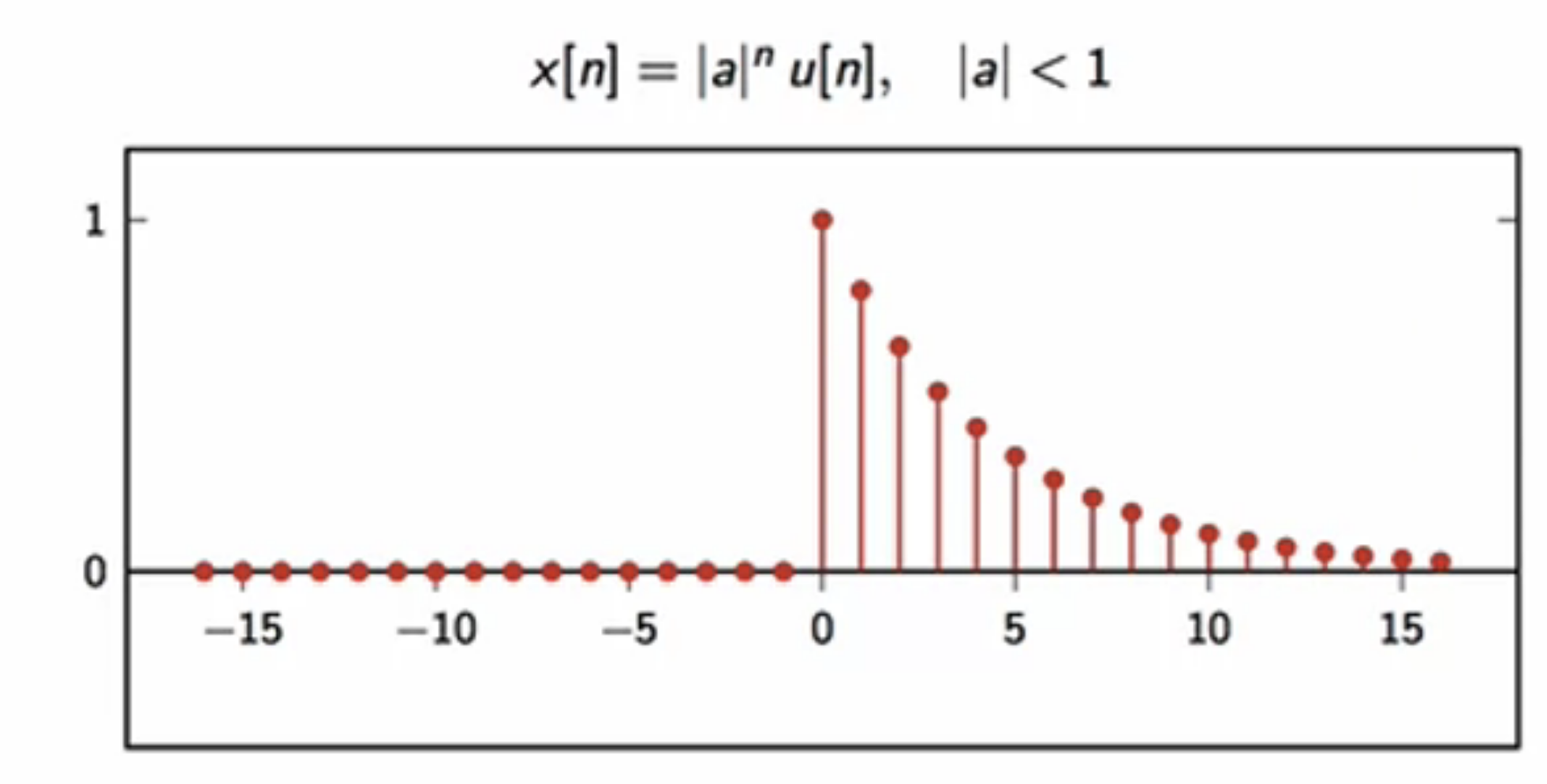
fig: discrete exponential decay

• sinusoid: $x\left[n\right]=sin({\omega }_{0}n+\theta )$
  • ${\omega }_0$: angular frequency $rad$
  • $\theta$: initial phase $rad$

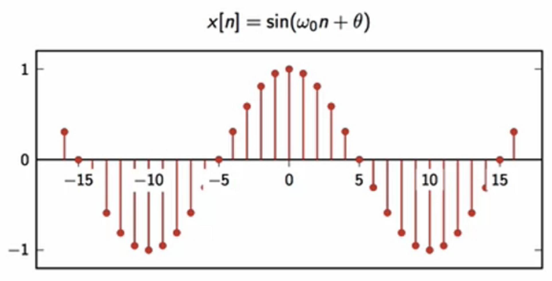
fig: discrete sinusoid

---

signal classes

• finite-length
• infinite length
• periodic
• finite-support

finite-length signals

• can only have $N$ samples
  • $N$: range of signal
  • $N$ is limited in finite-length signals
• notations:
  • sequence: $x\left[n\right],n=0,1,\dots ,N-1$
  • vector: $x=[x_0,x_1,\dots ,x_{N-1}{]}^T$
• practical entities
  • good for numerical packages

infinite-length signals

• can have infinite number of samples
• it is an abstraction
• useful for theorems that do not depend on the length of the data

periodic signals

• repetitive samples with a constant frequency
• notation: $\tilde{x}$ $x-tilde$
• $N$-periodic signals: $x\left[n\right]=\tilde{x}[n+kN];n,k,N\in Z$
  • data repeats every $N$ samples
  • same information as finite-length of length $N$
  • natural bridge between finite and infinite lengths

finite-support signals

• infinite length sequence
  • but only a finite number of non-zero sample
• notation: $\overline{x}$ $x-bar$
• $\overline{x}=x\left[n\right]$ if $0\le n\le N)else\text{(}x=0;n\in Z$
• same information as finite-length
• another bridge between finite and infinite length lengths

---

elementary signal operations

• scaling:
  • $y\left[n\right]=\alpha \cdot x\left[n\right]$
• sum:
  • $y\left[n\right]=x\left[n\right]+z\left[n\right]$
• product:
  • $y\left[n\right]=x\left[n\right]\cdot z\left[n\right]$
• delay (shift):
  • $y\left[n\right]=x[n-k],x\in Z$
  • output of operation is shifted by $k$ samples
  • care must be taken to append and prepend zeros to accommodate the shift
  • two types of delay:
    • finite-length is turned into finite-support
      • by adding zeros until $-\infty$ and $+\infty$
      • then shift is applied
    • make the finite-signal periodic:
      • samples circle around in the given range of $N$
• energy:
  • sum of the squares of all amplitudes of the signal
  • consistent with physical energy
  • many signals have infinite energy i.e. periodic signals
  • so not a great way to describe the energetic property of a signal

$$E_x=\sum _{n=-\infty }^{\infty }\left|x\right[n]{|}^2$$

• power:
  • a signal cannot have infinite power even if it’s energy is infinite
  • power is the rate of production of energy for a sequence
  • it is limit of the ratio of local energy in a window to the size of the window as N goes to infinity
  • for a periodic signal, the power is the ratio fo energy in one period to the length of the period

$$P_x=\underset{N\to \infty }{lim}\frac{1}{2N+1}\sum _{n=-N}^N\left|x\right[n]{|}^2$$

---

simple dsp applications

digital vs. physical frequency

• discrete time:
  • $n$: just a counter, no time dimension
  • periodicity: number of samples of one cycle of the pattern
• physical time:
  • frequency: $\text{Hz}\left(s^{-1}\right)$
  • periodicity: number of seconds of one cycle of the pattern

dsp lab: laptop/desktop

• a desktop computer is a signal processing lab for all practical purposes
• signals can be generated
  • visualed as plots
  • can be used to generate sounds
    • an analog-digital interface is needed for this
• a sound card is an interface that converts digital signals to analog
  • has a system clock of period $T_s$ seconds
  • discrete samples at $T_s$ intervals are sampled and converted to analog electrical signals
• a periodicity of $M$ samples in digital domain
  • becomes $M{T}_s$ seconds in the physical domain
  • frequency in physical domain $f=\frac{1}{M{T}_s}\text{Hz}$
• sampling rate for sound card: $F_s$
  • $T_s=\frac{1}{F_s}$
  • usually $F_s=48000\text{Hz}$; so $T_s\approx 20.8\mu s$
  • so, for $M=110\text{,}f\approx 440\text{Hz}$
  • and $M=\frac{F_s}{f}$
• dsp involves a few fundamental building blocks
  • adder block:
    • $x\left[n\right]+y\left[n\right]$ fig: adder block
  • scaler block:
    • $\alpha \cdot x\left[n\right]$ fig: scaler block
  • delay block:
    • $x\left[n\right]\to z^{-1}\to x[n-1]$
      • $\left(z^{-1}\right)$ means unit buffer
      • holds current value and send previously held value fig: unit delay (buffer) block
    • $x\left[n\right]\to z^{-N}\to x[n-N]$
      • $\left(z^{-N}\right)$ means $N$ samples buffer fig: N delay (buffer) block
• these blocks can be combined in any way to build arbitrarily complex circuitry for analysis or synthesis
  • an abstract implementation of dsp algorithm is first made
    • with the building blocks in a flow chart
    • can then be coded and executed in any language
  • example: moving average:
    • local average of a few samples
    • 2-sample moving average:
      • $y\left[n\right]=\frac{x\left[n\right]+x[n-1]}{2}$ fig: two-point moving average block
    • M sample moving average is an ubiquitous tool to smooth discrete signals
• feedback loop:
  • unit delay feedback loop
    • $y\left[n\right]=x\left[n\right]+\alpha x[n-1]$ fig: feedback loop with delay
  • introduces recursion in the algorithm: chicken-and-egg problem
  • to solve the particular problem feedback loop is applied to
    • set a start time $n_0$
    • assert zero initial conditions for input and output for all time before $n_0$
  • feedback loop for interest accumulation in a bank account:
    • assume interest rate 10% p.a.
    • interest accrual date: Dec 31
    • deposit/withdrawals in year $n$: $x\left[n\right]$
    • so balance (with accrued interest) at year-end is:
      • $y\left[n\right]=1.1y[n-1]+x\left[n\right]$
  • M-delay feedback loop:
    • $y\left[n\right]=x\left[n\right]+\alpha x[n-M]$ fig: M-samples delay feedback loop
    • equivalent to cascading unit delays in feedback branch
• Karplus-Strong Algorithm:
  • to synthesize plucked-string sound
  • algorithm: build a recursion loop with a delay $M$
    • $y\left[n\right]=x\left[n\right]+\alpha x[n-M]$
    • the number of samples controls the pitch of the output sound
  • input: finite support signal $\overline{x}\left[n\right]$
    • non-zero only for $0\le n<M$
    • this controls the timbre of the output
  • parameters to configure (knobs of the algorithm):
    • decay factor: $\alpha$
      • $\alpha =1$: no decay (100% feedback)
      • $\alpha =0$: extreme decay (0% feedback)
    • controls how sustained the sound is
  • run the algorithm on the input to generate output
  • a random valued $\left(\right[-1,1\left]\right)$ finite-support signal input was found to give best results
• Refactoring DSP operations:
  • DSP operations can get complex very quickly
  • refactoring them is an art that heavily aids building simple block diagrams
  • the simplified expressions are used for efficiency in analysis and synthesis

---

references

• Number Sets and Operation Symbols
• Sampling Theorem
• Karplus-Strong algorithm
• coursera dsp