[DSP] W04 - Sinusoidal Modulation

• in previous posts, calculating the spectrum of signals was explored
  • in most cases, this spectrum is not wideband: it is mostly limited around a certain range of frequencies
• depending on this range, different types of signals can be defined.
  • if most of the energy of a signal is concentrated around zero (resp. $-\pi$ or $\pi$), it is a lowpass (reps. highpass) signal
  • if the energy is concentrated somewhere in between, it is a bandpass signal

---

signal modulation

• fourier transform modulation theorem:
  • allows to transform a signal
• for example, a lowpass signal can be modulated into a bandpass signal
  • this operation can be reversed by demodulating
• this is obtained by simply multiplying the signal by a cosine at the adequate frequency
• having seen this theoretical result, it can be put to work on a practical application like tuning a guitar

categories based on energy concentration

• there are three broad categories according to where most of the spectral energy resides
  • lowpass signals (baseband signals)
  • highpass signals
  • bandpass signals

• lowpass signal: energy is mostly concentrated around the origin

  

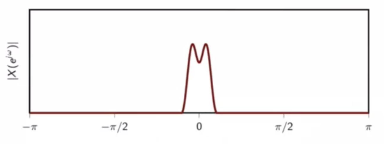
  fig: lowpass signal

• bandpass signal: energy is mostly concentrated around $-\pi$ and $\pi$)

  

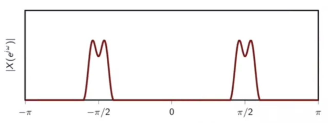
  fig: bandpass signal

• highpass signal: energy is mostly concentrated around $\frac{-\pi }{2}$ or $\frac{\pi }{2}$

  

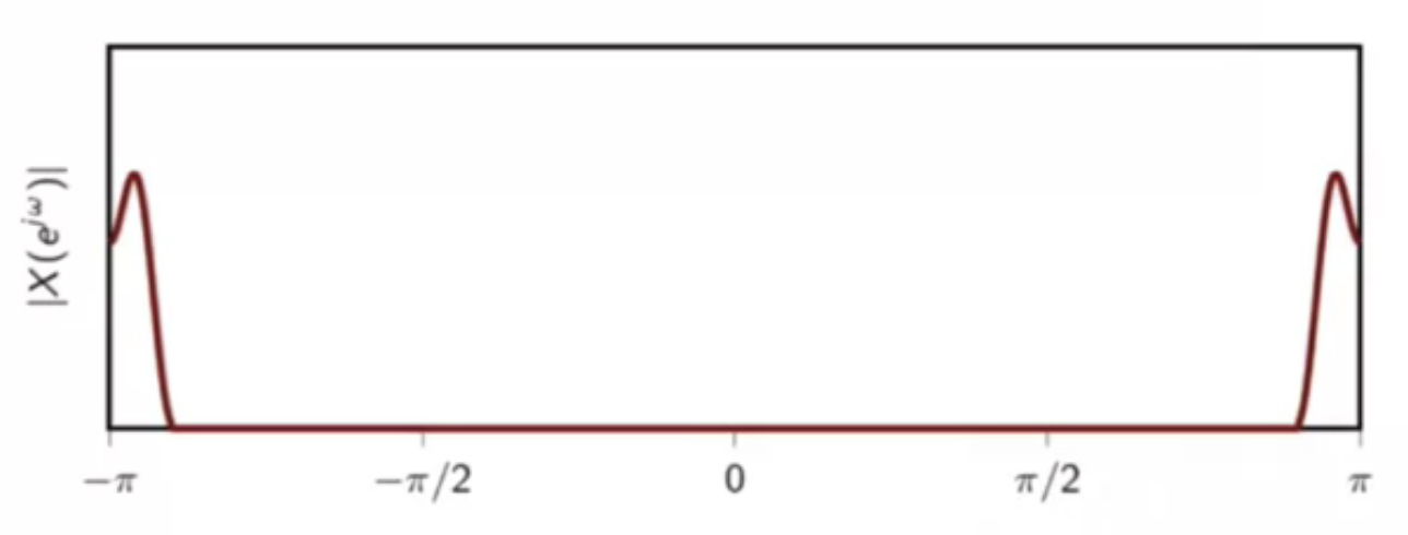
  fig: highpass signal

---

sinusoidal modulation

• this type of modulation is obtained by multiplying a signal $x\left[n\right]$ with a $\cos \left({\omega }_{c}n\right)$
  • ${\omega }_c$ is the carrier frequency

• to analyze the spectrum of this modulation, take DTFT: $$DTFT\left\{x\right[n\left]\cos \right({\omega }_{c}n\left)\right\}=DTFT\{\frac{1}{2}{e}^{j{\omega }_{c}n}x\left[n\right]+\frac{1}{2}{e}^{-j{\omega }_{c}n}x\left[n\right]\}=\frac{1}{2}[X\left(e^{j(\omega -{\omega }_c)}\right)+X\left(e^{j(\omega +{\omega }_c)}\right)]$$

• modulation, pictorially:

  

  fig: begin with source signal

  

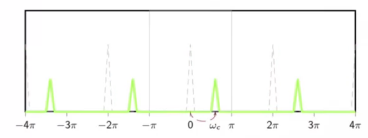
  fig: apply ${\omega }_c$ shift

  

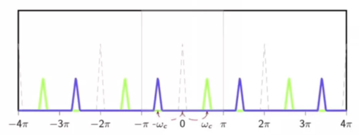
  fig: apply $-{\omega }_c$ shift

  

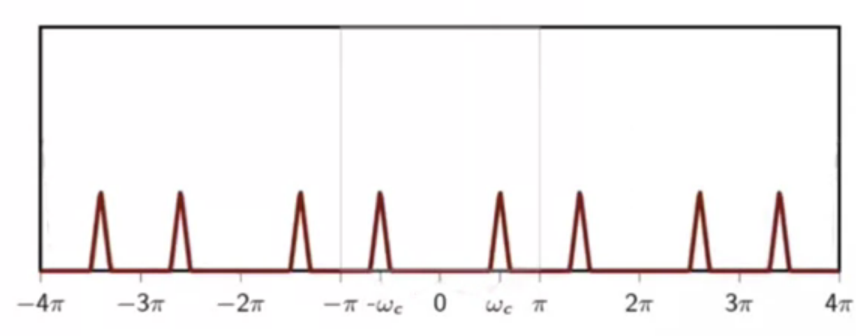
  fig: modulated signal

• when modulation frequency is too large:
  • when $-{\omega }_c$ is close to $\pi$ or $-\pi$
  • the original signal loses shape and information is lost

application of modulation

• modulation brings the baseband signal to the transmission band
  • i.e. voice to radio frequencies
• demodulation at the receiver brings it back
  • i.e. radio to voice
• voice and music are lowpass signals
  • energy is lost during transmission over very short distances
• radio channels are bandpass signals
  • their modulation frequencies are higher, else they lose the information embedded in them through interference
• radio waves are carrier signals and are modulated with audio sources
• then, they are transmitted from source to destination
• at the destination, the source audio is retrieved from the carrier by demodulation

---

sinusoidal demodulation

• simply multiply the received signal by the carrier again to get the original signal $$y\left[n\right]=x\left[n\right]cos\left({\omega }_{c}n\right)$$ $$Y\left(e^{j\omega }\right)=\frac{1}{2}[X\left(e^{j(\omega -{\omega }_c)}\right)+X\left(e^{j(\omega +{\omega }_c)}\right)]$$

$$DTFT\left\{y\right[n]\cdot 2\cos ({\omega }_{c}n)=Y(e^{j(\omega -{\omega }_c)})+Y(e^{j(\omega +{\omega }_c)})=\frac{1}{2}[X(e^{j(\omega -{\omega }_c)})+X(e^{j\omega })+X(e^{j\omega })+X(e^{j(\omega +{\omega }_c)})]=X(e^{j\omega })+\frac{1}{2}[X(e^{j(\omega -{\omega }_c)})+X(e^{j(\omega +{\omega }_c)})]$$

• demodulation, pictorially:

  

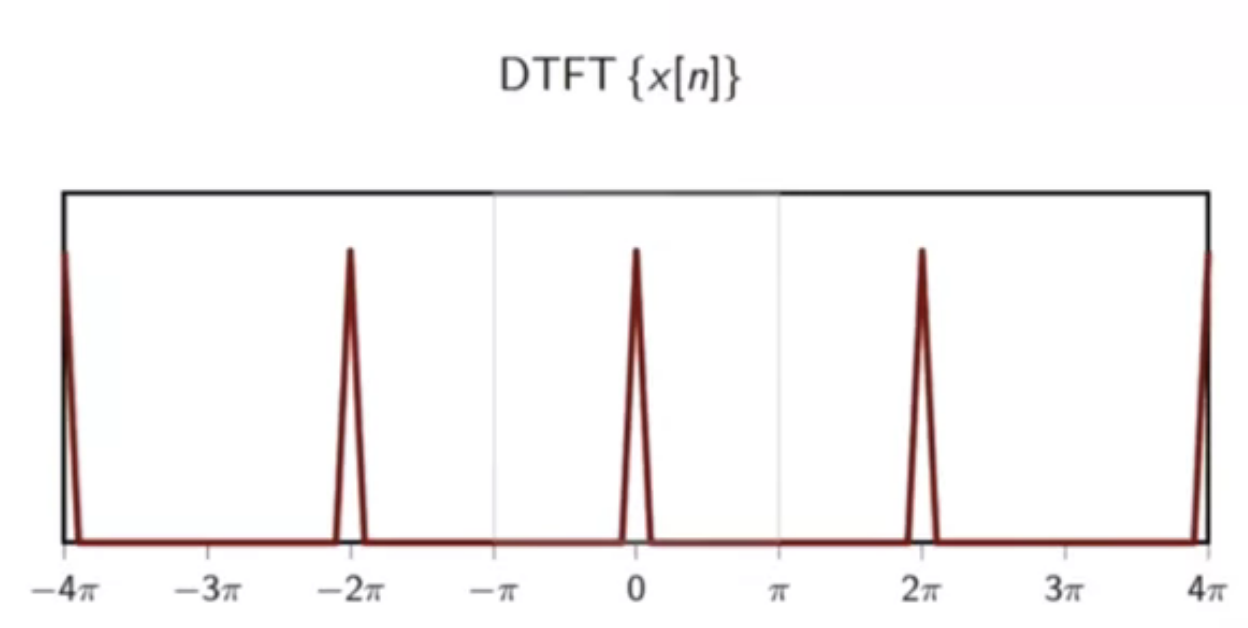
  fig: source signal

  

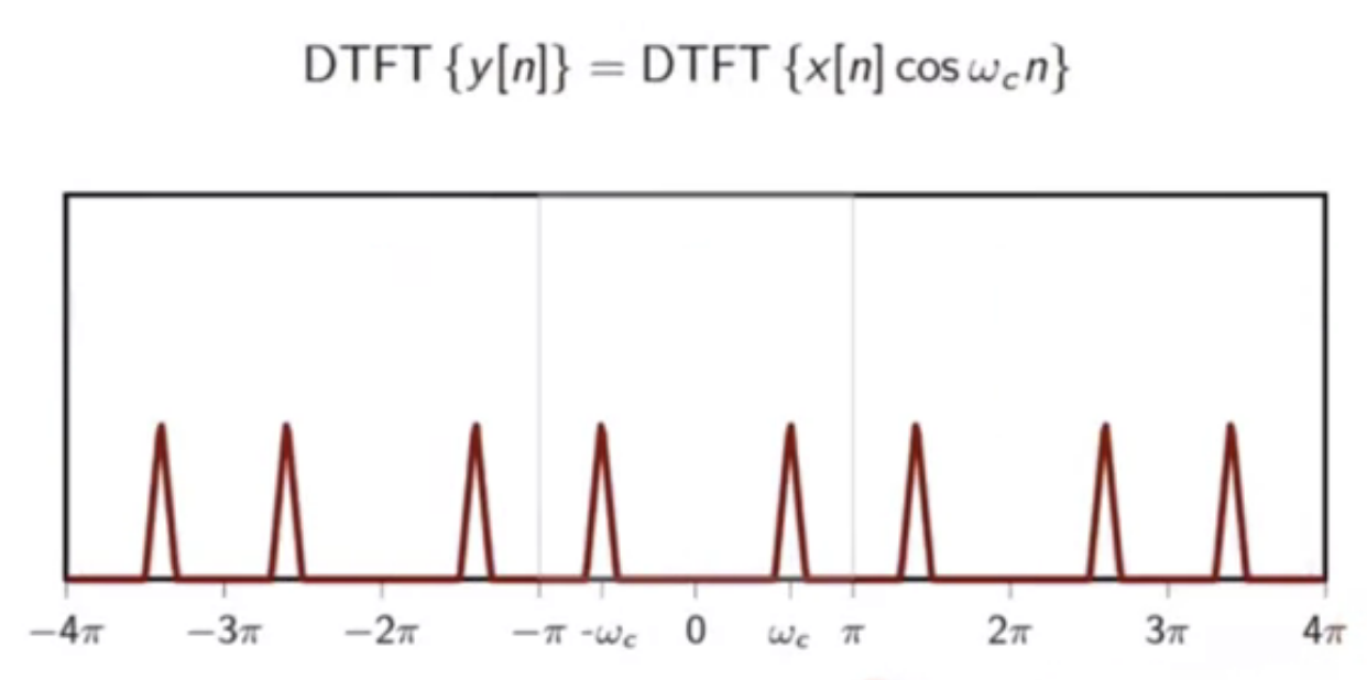
  fig: modulated version of signal

  

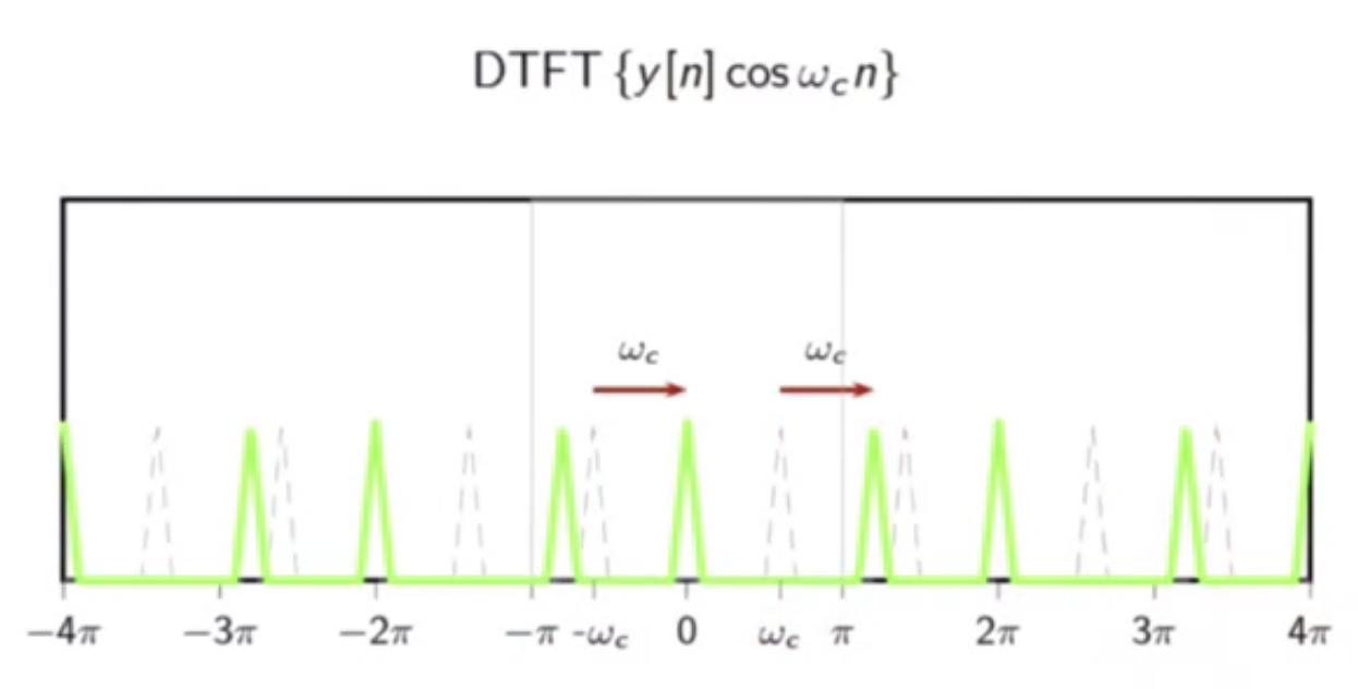
  fig: signal shifted to right

  

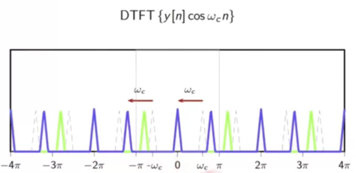
  fig: signal shifted to left

  

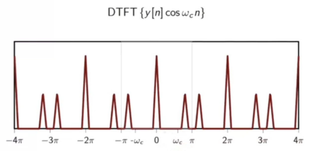
  fig: sum of shifted signals

  

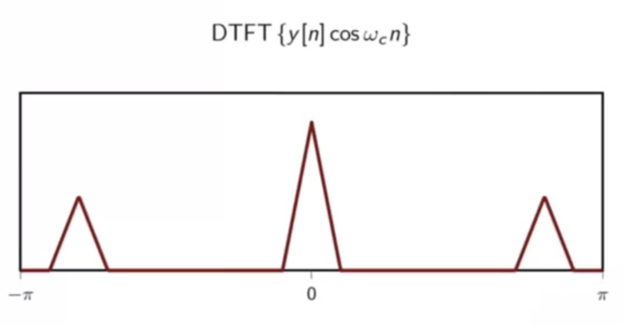
  fig: demodulated signal

• the baseband signal can be recovered
• but some spurious high-frequency components exist
  • those will have to be filtered out

---

application: guitar tuning

• problem statement:
  • reference sinusoid: frequency ${\omega }_0$
  • tunable sinusoid: frequency $\omega$
• tuning:
  • make $\omega ={\omega }_0$ “by ear”

procedure

1. bring $\omega$ close to ${\omega }_0$
2. when $\omega \approx {\omega }_0$, play both sinusoids together
3. trigonometry can then be used:
   • $x\left[n\right]=\cos \left({\omega }_{0}n\right)+\cos \left(\omega n\right)$
   • $=2\cos \left(\frac{{\omega }_0+\omega }{2}n\right)+\cos \left(\frac{{\omega }_0-\omega }{2}n\right)$
   • $\approx 2\cos \left({\Delta }_{\omega }n\right)\cos \left({\omega }_{0}n\right)$

procedure analysis

• in $x\left[n\right]\approx 2\cos \left({\Delta }_{\omega }n\right)\cos \left({\omega }_{0}n\right)$
  • error signal: $2\cos \left({\Delta }_{\omega }n\right)$
  • modulation at ${\omega }_0$ $\cos \left({\omega }_{0}n\right)$
• when $\omega \approx {\omega }_0$, error is too low to be heard
  • so the modulation signal multiplication brings it up to hearing range
  • it is perceived as amplitude oscillations of carrier frequency
• pictorially:
  • red signal is the carrier frequency
  • blue is the audible beats heard

  

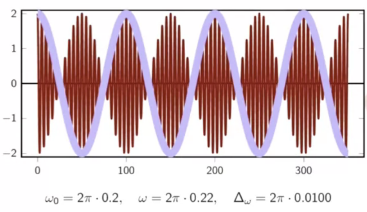
  fig: time domain signals - beat frequency

  

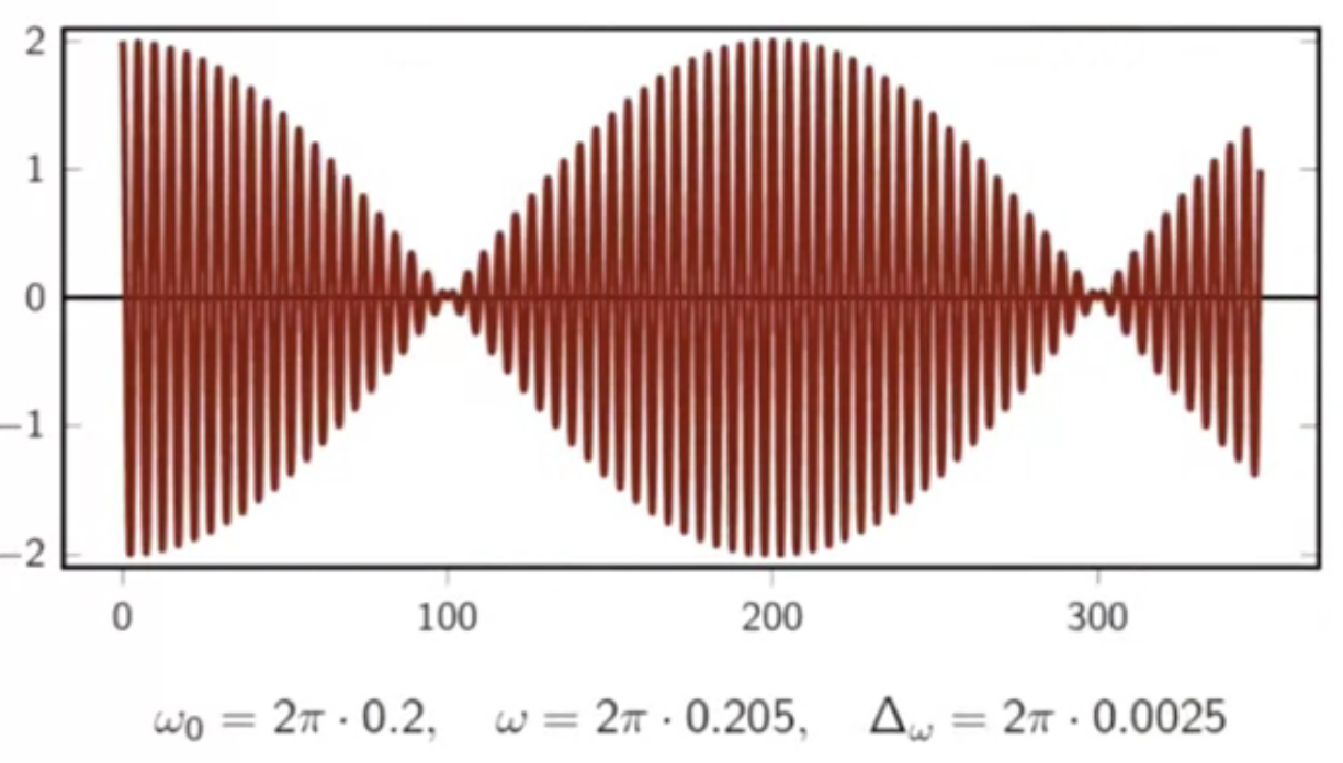
  fig: time domain signals - slower beat frequency

  

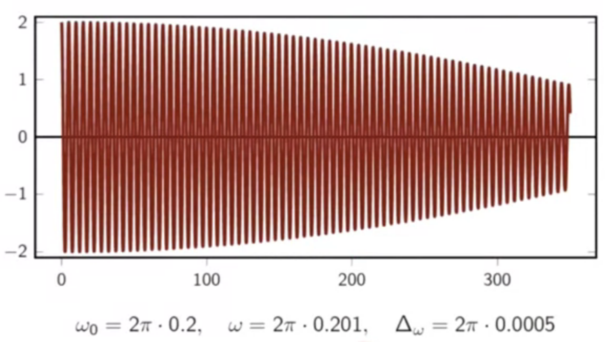
  fig: almost nil beat frequency