[DSP] W05 - Filters
contents
- signal processing
- linear filters
- impulse response
- convolution
- filtering applications
- filter classification
- filter stability
- references
signal processing
- signal processing is where a signal is manipulated to transform it into another signal after analysis
- there are many ways to skin a signal
filters
- this post is focussed on linear time-invariant filters
- LTI filters
- these are simple, yet powerful devices that have been around a long time i.e. since analog electronics have existed
- example:
- boosting bass on stereo system
- dim treble on stereo system
- in the digital signal world, the implementation of these filters is simpler on general purpose architecture
- goals:
- define the filter paradigm
- filter characterization
- ideal filters
- implementing filters
- filter design (and beyond ideal filters)
- z-transform in filter design
- define the filter paradigm
- this covers the very basics of filters in dsp
linear filters
- SISO: a single-input-single-output signal processor takes in a single input, operates on it and outputs the resulting signal
fig: dsp SISO block
- (x[n]): input signal
- (y[n]): output signal
- ( \mathcal{H} ): operator block
- where: ( y[n] = \mathcal{H}{ x[n] } )
- this operation (\mathcal{H} ) can be anything and is limitless -so operation modified as per dsp application
- for a filter, this operation has some restrictions fig: LTI SISO filter requirements
linearity
- operation on sum of two signals must result in the same as the sum of operation result separately on the two signals \[ \mathcal{H} { \alpha x_1[n] + \beta x_2[n] } = \alpha \mathcal{H} { x_1[n] } + \beta \mathcal{H} { x_1[n] } ]
- addition and scalar multiplication are covered under linearity
time-invariance
- the operator result for a given signal must be same whenever it is applied, independent of time \[ y[n] = \mathcal{H} { x[n] } \Leftrightarrow \mathcal{H} { x[n - n_0] } = y[n - n_0] ]
causal system
- this is an optional requirement
- helps real-time LTI system implementation
- system depends only on the input and output values of the past
- along with present input
- physical or non-anticipatory system
\[ y[n] = \mathcal{H}( x[n], x[n-1], x[n-2], \ldots, y[n-1], y[n-2], \ldots )
]
- here: ( \mathcal{H}(\cdot) ) is a linear function of its arguments
impulse response
- impulse response of filter (h[n]):
- the output of a filter when the input is ( \delta )
- ( h[n] = \mathcal{H}{\delta[n]})
- impulse response fully characterizes the behavior of an LTI system
- this is because all arbitrary inputs can be expressed in terms of a (\delta) signal
- so, knowing the response of a filter to the delta signal, along with linearity conditions, filter response for any arbitrary signal can be computed
example
- consider filter characterized by ( h[n] = \alpha^n u[n] ) : fig: impulse response ( h[n] = \alpha^n u[n] )
- here ( h[n] = \mathcal{H} { \delta[n]} )
- an arbitrary signal is fed to the filter: fig: arbitrary input signal to filter whose ( h[n] ) is known
- all signals can be represented in terms of the ( \delta ) function \[ x[n] = \sum_{k=-\infty}^{\infty} x[k] \delta[n-k] ]
- since all signals can be represented in terms of the ( \delta ) function, above input signal is cast in terms of the (\delta ) signal to obtain
\[ x[n] = 2\delta[n] + 3\delta[n-1] + \delta[n-2] ]
- to compute the output ( y[n] ) of the filter for the above input
\[ \begin{align}
y[n] & = \mathcal{H} { x[n] }
& = \mathcal{H} { 2\delta[n] + 3\delta[n-1] + \delta[n-2] }
& = \mathcal{H} { 2\delta[n] } + \mathcal{H} { 3\delta[n-1] } + \mathcal{H} { \delta[n-2] }
& = 2 \mathcal{H} { \delta[n] } + 3 \mathcal{H} { \delta[n-1] } + \mathcal{H} { \delta[n-2] }
& = 2 h[n] + 3 h[n-1] + h[n-2]
\end{align} ]
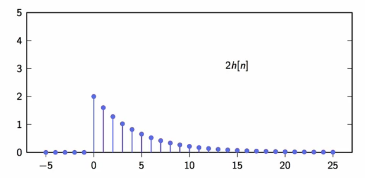
fig: first filter output component ( 2 h[n] )
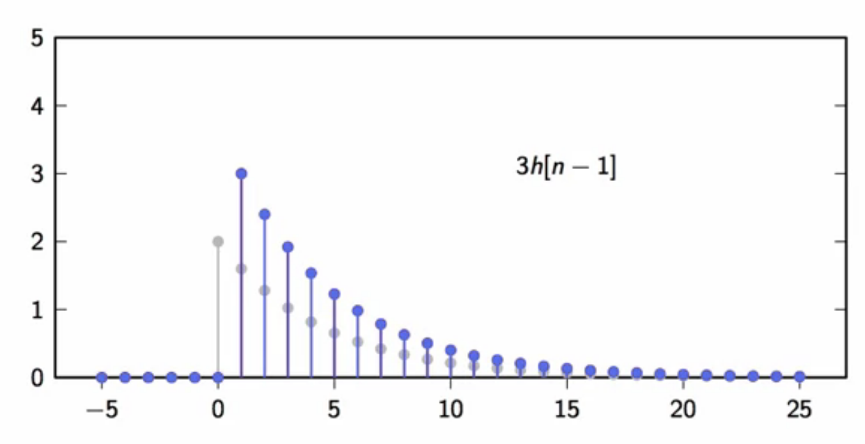
fig: second filter output component ( 3 h[n-1] )
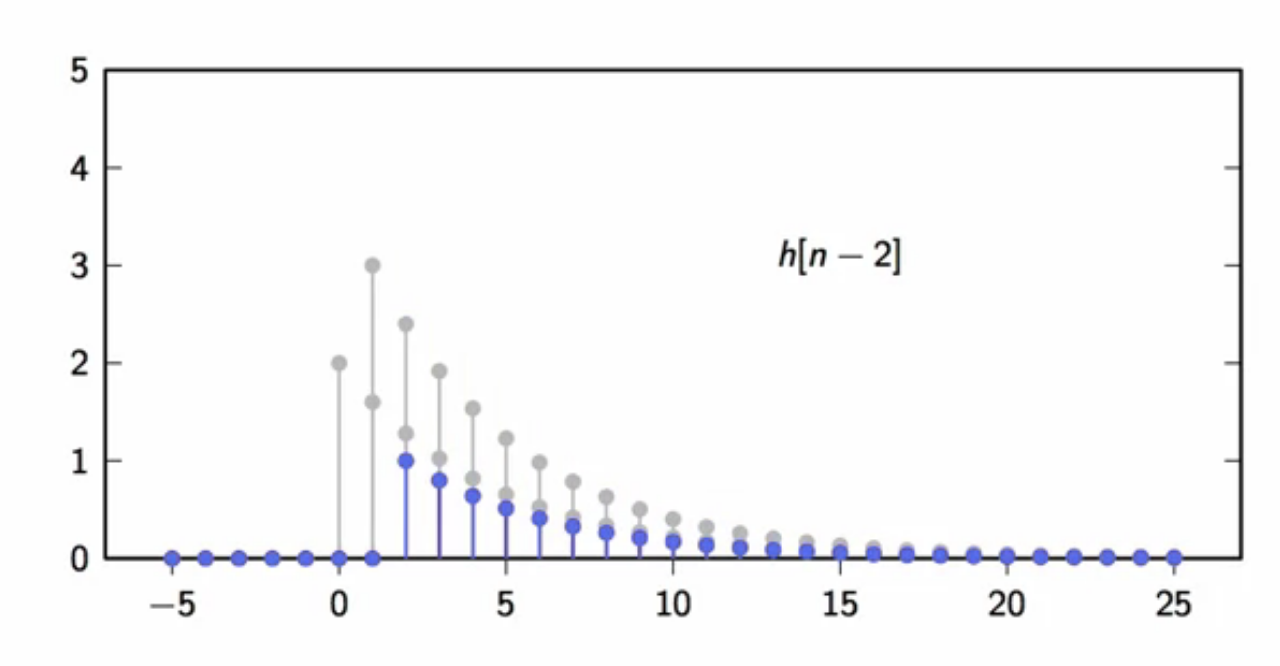
fig: third filter output component ( h[n-2] )
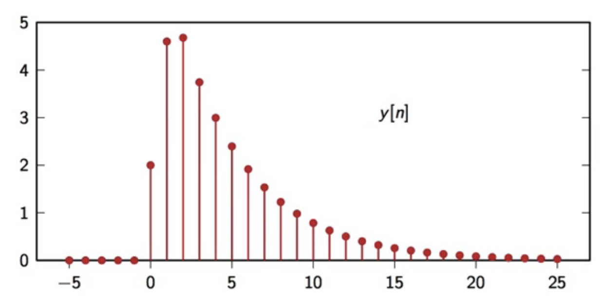
fig: sum of components of filter output ( y[n] )
- so, output of a filter for any arbitrary signal can be expressed in terms of the impulse response (h[n])
\[ \begin{align}
y[n] & = \sum_{k = -\infty}^{\infty} x[k] h[n-k]
y[n] & = x[n] * h[n] \end{align} ] - above filter operation is called convolution
convolution
\[ \begin{align}
x[n] * h[n] & = \sum_{k = -\infty}^{\infty} x[k] h[n-k]
\end{align}
]
inputs of convolution:
- a sequence: (x[m] )
- a second sequence: ( h[m] )
convolution procedure:
- time-reversed: ( h[m] )
- at each step (n) (from (-\infty ) to (\infty))
- center the time-reversed ( h[m] ) in ( n )
- i.e. shift by (-n)
- compute the inner product of the two signals
- center the time-reversed ( h[m] ) in ( n )
convolution properties
- linearity and time invariance
- commutativity:
- ( x[n] _h[n] = (h_n)[n] )
- filter order doesn’t matter in a cascade of filters, they can be switched
- associativity: (for absolutely- and square-summable sequences)
- ( (x h) w)[n] = (x (h w))[n] )
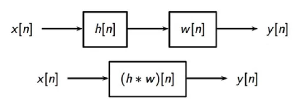 fig: associativity - filters can be lumped in a filter cascade
- ( (x h) w)[n] = (x (h w))[n] )
applications
- auralization
- apply room-impulse-response to sounds in virtual reality
- used in music production to simulate environment effects
- dry sounds are convolved with room-impulse-responses to create mental imagery in sounds
- realistic impulses are only approximations to dirac-delta function
- so the room-impulse-responses convolutions are not perfect
- shape of an environment can be reproduced in sound
- if the room is not too complex
- involves localization of multiple sources
- multiple sound sensors can localize the room-response better as they can localize more features of the room
filtering applications
- there are several applications of filtering, noise filtering is one of them
- consider the scenario where a smooth signal is measured
- due to the measurement process, the measured value has a perturbation that affects the smoothness of the measured signal
- this leads to a noisy signal fig: noisy signal resulting from a measurement
- noise filtering:
- removing noise from an otherwise smooth signal
- apply dsp to get as close as possible to the original smooth signal
- examples of noise filters (de-noising):
- moving-average
- leaky integrator
moving-average filter
- replace each sample of the input sequence by the local average
- 2-pt moving-average filter: \[ y[n] = x[n] + \frac{x[n-1]}{2} ] fig: measured signal filtered with 2-pt moving-average
- more general moving-average filter \[ y[n] = \frac{1}{M} \sum_{k=0}^{M-1}x[n - k] ]
<img class="plot mx-auto text-center img-fluid" src="/images/uploads/noise-filter-02.png" alt="nf-02">

*fig: measured signal filtered with 4-pt moving-average*
{: style="font-size: 80%; text-align: center;"}

<img class="plot mx-auto text-center img-fluid" src="/images/uploads/noise-filter-03.png" alt="nf-03">

*fig: measured signal filtered with 12-pt moving-average*
{: style="font-size: 80%; text-align: center;"}

<img class="plot mx-auto text-center img-fluid" src="/images/uploads/noise-filter-04.png" alt="nf-04">

*fig: measured signal filtered with 100-pt moving-average*
{: style="font-size: 80%; text-align: center;"}

- the 100-pt moving-average is very smooth, but the output has a delay with respect to the input
- this is because a large amount of input samples have to accumulated before the average can be computed for a point
- so delay is the price to pay for more a more smoothed out signal
moving-average - impulse response
- (M)-pt moving-average filter characterization
- done with impulse response input
\[ \begin{align}
h[n] & = \frac{1}{M} \sum_{k=0}^{M-1} \delta [n-k]
& = \Bigg { \begin{matrix} \frac{1}{M} & \text{ for } 0 \leq n < M \ 0 & \text{ otherwise } \end{matrix}
\end{align} ] fig: impulse response (h[n]) of (M)-pt moving-average filter
- done with impulse response input
\[ \begin{align}
h[n] & = \frac{1}{M} \sum_{k=0}^{M-1} \delta [n-k]
moving-average - analysis
- proportional to ( M )
- smoothing effect
- number of operations for computing each output
- storage and memory used
- delay of output w.r.t signal to be smoothed
- here, while better smoothing is desired, the cost gets in the way
- so another method is explored to reduce smoothing costs of a signal, while keeping the smoothing effect high
first-order recursion
- technique to reduce the computation power and memory needed for large-pt moving-average
- derivation:
- moving-average of (M) points:
\[ \begin{align}
y_M[n] & = \frac{1}{M} \big ( x[n] + x[n-1] + x[n-2] + \ldots + x[n - M + 1] \big )
\end{align} ] - rearranging:
\[ \begin{align}
y_M[n] & = \frac{1}{M} x[n] + \frac{1}{M} \big ( x[n-1] + x[n-2] + \ldots + x[n - M + 1] \big )
\end{align} ] - here, the second term of the sum has ( M-1 ) terms
- this is similar to the moving-average of (M-1) terms
\[ \begin{align}
y_{M-1}[n-1] & = \frac{1}{M} \big ( x[n-1] + x[n-2] + \ldots + x[n - M + 1] \big )
\end{align} ]- i.e. moving-average over ( M - 1 ) points, delayed by one
- moving-average of (M) points:
\[ \begin{align}
y_M[n] & = \frac{1}{M} \big ( x[n] + x[n-1] + x[n-2] + \ldots + x[n - M + 1] \big )
- formally:
[ \begin{align}
y_M[n] & = \frac{1}{M} \sum_{k=0}^{M-1} x[n-k]
y_M[n - 1] & = \frac{1}{M} \sum_{k=1}^{M-1} x[n-k]
y_{M-1}[n-1] & = \frac{1}{M-1} \sum_{k=1}^{M-1} x[n-k]
\end{align} ]- also, summing only first ( M-1 ) samples:
[ \begin{align}
\sum_{k=0}^{M-1} x[n-k] = x[n] + \sum_{k=1}^{M-1} x[n-k]
\end{align} ] - comparing it to the above set of equations:
[ \begin{align}
My_M[n] = x[n] + (M-1)y_{M-1}[n-1]
\end{align} ] - this relates the moving-average between (M ) points ( My_M[n] ) and the moving-average of (M - 1 ) points delayed by 1 (y_{M-1}[n-1])
- rearranging for (y_{M}[n]):
\[ \begin{align}
y_M[n] = \frac{1}{M} x[n] + \frac{M-1}{M}y_{M-1}[n-1]
\end{align} ] - introducing ( \lambda = \frac{M-1}{M} )
[ \begin{align}
y_M[n] = \lambda y_{M-1}[n-1] + (1-\lambda) x[n]
\end{align} ]
- also, summing only first ( M-1 ) samples:
[ \begin{align}
\sum_{k=0}^{M-1} x[n-k] = x[n] + \sum_{k=1}^{M-1} x[n-k]
leaky integrator
- in a moving-average filter, when (M) is large, assume:
\[ \begin{align}
y_{M-1}[n-1] & \approx y_M[n]
\lambda & \approx 1 \end{align} ]- i.e. average doesn’t change much by excluding one data point
- this assumption is applied to the recursive moving-average filter
- which yields the leaky integrator filter
\[ \begin{align}
y[n] = \lambda y[n-1] + (1-\lambda) x[n]
\end{align} ]
- which yields the leaky integrator filter
\[ \begin{align}
y[n] = \lambda y[n-1] + (1-\lambda) x[n]
- this filter is recursive:
- previous output value is used to compute current value
- de-noising for various (\lambda ) values:
fig: measured signal filtered with (\lambda = 0.2) leaky-integrator
fig: measured signal filtered with (\lambda = 0.5) leaky-integrator
fig: measured signal filtered with (\lambda = 0.8) leaky-integrator
fig: measured signal filtered with (\lambda = 0.98) leaky-integrator
leaky integrator - analysis
- closer the value of (\lambda ) to (1), more the smoothing
- ( \lambda ) values very close to (1) provides smoothing power similar to a moving-average filter with large (M)
- so, the leaky integrator is a special case of a moving-average filter
- for when the (M) values are large
- each average requires only three operations
- average at every point is ( y[n] = \lambda y[n-1] + (1-\lambda)x[n] )
- two multiplications, one addition
- number of operations are independent of ( \lambda ) value
- so high smoothing power at a fixed price
leaky integrator - impulse response
- leaky integrator with delta input \[ y[n] = \lambda y[n-1] + (1-\lambda)\delta[n] ]
- impulse response equation and plot
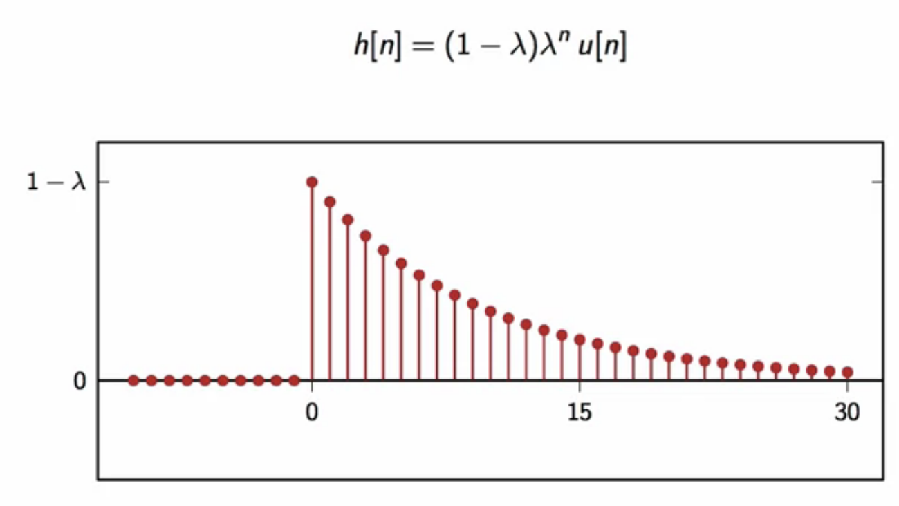
fig: leaky-integrator impulse response
non-leaky integrator comparison
- discrete-time integrator (non-leaky):
\[ y[n] = \sum_{k=-\infty}^{\infty} x[k]
]
- this is a boundless accumulator
- which is essentially a discrete-time integral
- this discrete-time integrator can be rearranged: \[ y[n] = y[n-1] + x[n] ]
- comparing to the leaky integrator equation:
\[ y[n] = \lambda y[n-1] + (1- \lambda) x[n]
]
- the first term here is the scaled by (\lambda)
- so only a percent of the past value is kept in the present value
- the rest is leaked out, or forgotten
- the leaked out portion ((1-\lambda)) is filled with current input
- the second term is the current input scaled by ((1-\lambda))
- the forgotten percent is replaced by an equal percent from the new
- the sum of there two fraction is fed to the accumulator as the current value
- so, the leaky integrator filter is similar to a discrete-time integrator, but
- has leak factor ( \lambda ) that sets accumulated past values percentage to be kept
- the rest is leaked
- the leak replace factor (1 - \lambda ) replaces leaked with an equal percent of current input
- has leak factor ( \lambda ) that sets accumulated past values percentage to be kept
- use only ( \lambda < 1) to prevent explosion of accumulation
filter classification
- filters can be classified according to their impulse-response shape in the time domain
- Finite Impulse Response Filters (FIR)
- Infinite Impulse Response Filters (IIR)
- Causal Filters
- Non-causal Filters
FIR filters
- filter’s impulse response has finite-support (with an infinite response)
- only a finite number of samples are involved in the computation of each output sample
- moving-average filter is an FIR filter
- only (M) samples are non-zero and are involved in computation
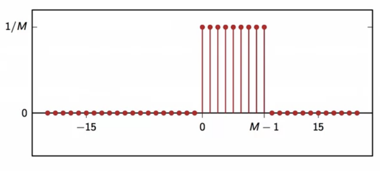
fig: FIR filter example - moving-average filter
IIR filters
- filter’s impulse response has infinite support
- a potentially infinite number of samples are involved in the computation of each output sample
- leaky integrator filter is an IIR filter
- recursive filters involve infinite samples
- surprisingly, in many cases the computation can still be performed in a finite-amount of steps
- a leaky integrator filter output can be computed with only three operations
- ideal filters are an exception
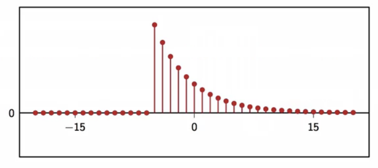
fig: IIR filter example - leaky integrator filter
causal vs. non-causal
- causal:
- ony past samples w.r.t present are involved in the output of filter
- impulse response is zero for (n < 0 )
- they can run on-line (real-time) since only past values are used
- physical filters
- the moving-average filter is a causal filter fig: causal filter example - moving-average filter
- noncasual:
- impulse response is non-zero for some (or all) ( n < 0 )
- is used for static (off-line) dsp, since future values are needed to compute current filter output
- used in scenarios where the whole data-set is available before dsp is applied
- batch processing of images is an example
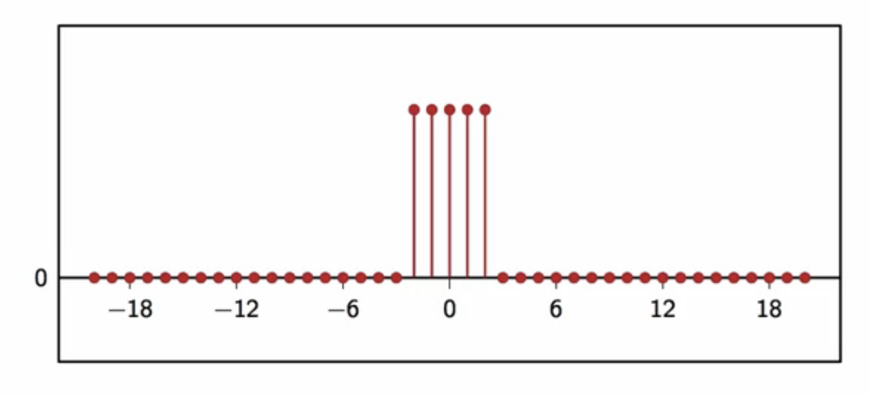
fig: noncausal filter example - zero centered moving-average filter
filter stability
- main goal:
- avoid filter “explosions” if the input is nice
- is a system is stable, it will not behave unexpectedly when its input is well-behaved
BIBO stability
- in dsp context, a well-behaved signal is a bounded signal
- ( \vert x[n] \vert < M ) for all (n)
- a signal whose maximum excursion is known
- Bounded-Input Bounded-Output system:
- system output is bounded when its input is bounded
fundamental filter stability theorem
- a filter is BIBO stable if and only if its impulse response is absolutely summable
- absolutely summable: sum of magnitudes is not infinity
- necessary and sufficient condition for stability
- FIR filters are always stable
- IIR filter stability has to be checked explicitly with its impulse response
- leaky-integrator filter stability is guaranteed only for (\vert \lambda \vert < 1 )
- indirect methods to assess filter stability exist
- without going through impulse response explicitly