[DSP] W05 - Frequency Response of Filters

contents

• frequency domain
  • eigen-sequences
  • convolution theorem
• denoising - frequency domain
  • magnitude analysis
  • phase analysis
• moving-average filter
  • moving average - magnitude response
  • moving average - phase response
• leaky-integrator filter
  • leaky integrator - magnitude response
  • leaky integrator - phase response
  • combined response
• karplus-strong algorithm
  • convolution in k-s algorithm

---

frequency domain

• filter impulse response is a time-domain attribute of a filter
• filters in the frequency domain are explored below
• if a complex exponential is processed with an LTI filter, the frequency of the phase doesn’t change
  • the output signal may only have an amplitude change and/or a phase shift
• the frequency response of a filter is an important characteristic of a filter in the frequency domain
• the moving-average filter, leaky-integrator filter and the karplus-string algorithm will be explored in the frequency domain

eigen-sequences

• consider a complex exponential: ( e^{j\omega_0 n} )
• input this to a filter characterized by impulse response (h[n]) \[ h[n] = \mathcal{H} { \delta[n] }
  ]
• output of a filter in terms of the impulse response (h[n]): \[ \begin{align} y[n] & = x[n] * h[n] \end{align} ]
• here: (x[n] = e^{j\omega_0 n} )
• so filter output can be written as: \[ \begin{align} y[n] & = e^{j\omega_0 n} h[n] _
  & = h[n] e^{j\omega_0 n} _
  _& = \sum{k = -\infty}^{\infty} h[k] e^{j\omega_0 (n - k)} & \rightarrow \text{ expansion of convolution } _
  & = e^{j\omega_0 n} \sum{k = -\infty}^{\infty} h[k] e^{-j \omega_0 k} & \rightarrow \text{ input, scaled by a DTFT }
  & = e^{j\omega_0 n} H(e^{j\omega_0}) & \rightarrow H(e^{j\omega_0}) = DTFT{h[n]}
  \end{align} ]
• here, the output of the filter is
  • the input scaled by
  • the DTFT @ the input signal frequency of the impulse response
• so, an LTI filter cannot change the frequency of the input \[ e^{j \omega_0 n} H(e^{j \omega_0}) = \mathcal{H} { e^{j \omega_0 n} } ]
  • in other words, complex exponentials are eigen-sequences of LTI systems

magnitude and phase

• consider a complex exponential input to an LTI filter
  • expresssed as ( \mathcal{H} { e^{j \omega_0 n} } )
• the output is given by:
  • ( \mathcal{H} { e^{j \omega_0 n} } = e^{j \omega_0 n} H(e^{j \omega_0}) )
• assume DTFT of filter impulse response ( H(e^{j \omega_0}) = Ae^{j \theta} )
  • (A \in \mathbb{R})
  • (\theta \in [-\pi,\pi])
• with this assumption, output of the LTI filter is: \[ \mathcal{H} { e^{j \omega_0 n} } = A e^{j(\omega_0 n + \theta}) ] - A: output amplitude - if ( A > 1 ): amplification - if ( 0 \leq A < 1 ): attentuation - (\theta): output phase shift - if ( \theta < 0 ): delay - if ( \theta > 0 ): advancement

convolution theorem

• answers the question:
  • what is the DTFT of two sequences: \[ DTFT{x[n] * h[n]} = ? ]
  • i.e. the DTFT of the output of a filter
• DTFT of (x[n]) shows
  • how to build (x[n]) from a set of complex exponential basis functions
  • any signal is made of infinitely many sinusoidal components of the form \[ X(e^{j \omega})e^{j \omega n} ]
  • deriving the dTfT of convolution of two signals: \[ \begin{align} DTFT { x[n] h[n] } & = \sum{n=-\infty}^{\infty} (x_h)[n] e^{-j\omega n}
    & = \sum_{n=-\infty}^{\infty} \sum_{k=-\infty}^{\infty} x[k] h[n-k] e^{-j\omega n}
    & = \sum_{n=-\infty}^{\infty} \sum_{k=-\infty}^{\infty} x[k] h[n-k] e^{-j\omega (n-k)} e^{-j\omega k}
    & = \sum_{k=-\infty}^{\infty} x[k] e^{-j\omega k} \sum_{n=-\infty}^{\infty} h[n-k] e^{-j\omega (n-k)}
    & = H(e^{j\omega}) X(e^{j\omega}) \end{align} ]
• so the DTFT of a filter output is equal to the product of the input DTFT and the filter’s impulse response DTFT
  • the DTFT of the impulse response is also called the frequency response of the filter

frequency response

• the fourier transform of filter impulse response is the frequency response of a filter
• DTFT of filter impulse response determines the frequency characteristic of a filter \[ H(e^{j\omega}) = DTFT { h[n] } ]
• magnitude and the phase response can be separately analysed

magnitude response

• amplification: ( \vert H(e^{j\omega}) \vert > 1 )
• attenuation: ( \vert H(e^{j\omega}) \vert < 1 )

phase response

• more complex to qualify
• overall delay and shape changes are quantified by the phase response
• allows to asses if filter will change the shape of the input or not
• DTFT of the output of a LTI filter is equal to the product of the DTFT of its input and the DTFT of its impulse response

---

denoising - frequency domain

• consider the scenario where a smooth signal is measured
  • due to the measurement process, the measured value has a perturbation that affects the smoothness of the measured signal
  • this leads to a noisy signal

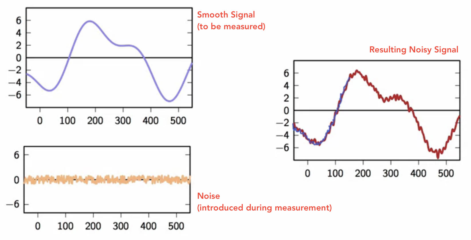
fig: noisy signal resulting from a measurement - time domain

• the noisy signal spectrum is analyzed in the frequency domain

magnitude analysis

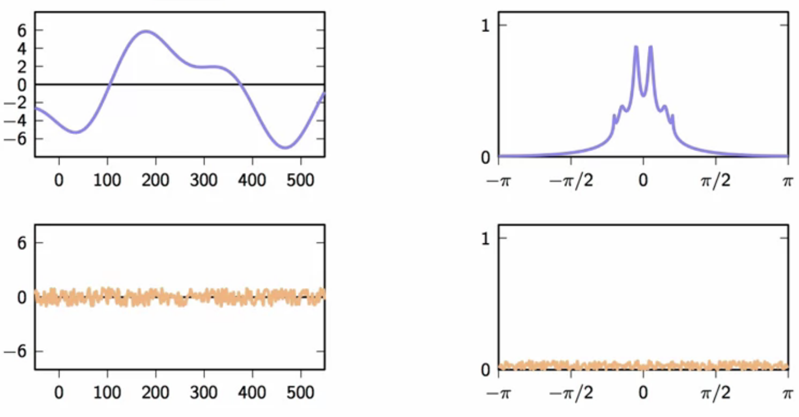
fig: left col - time domain; right col - frequency domain (DTFT)

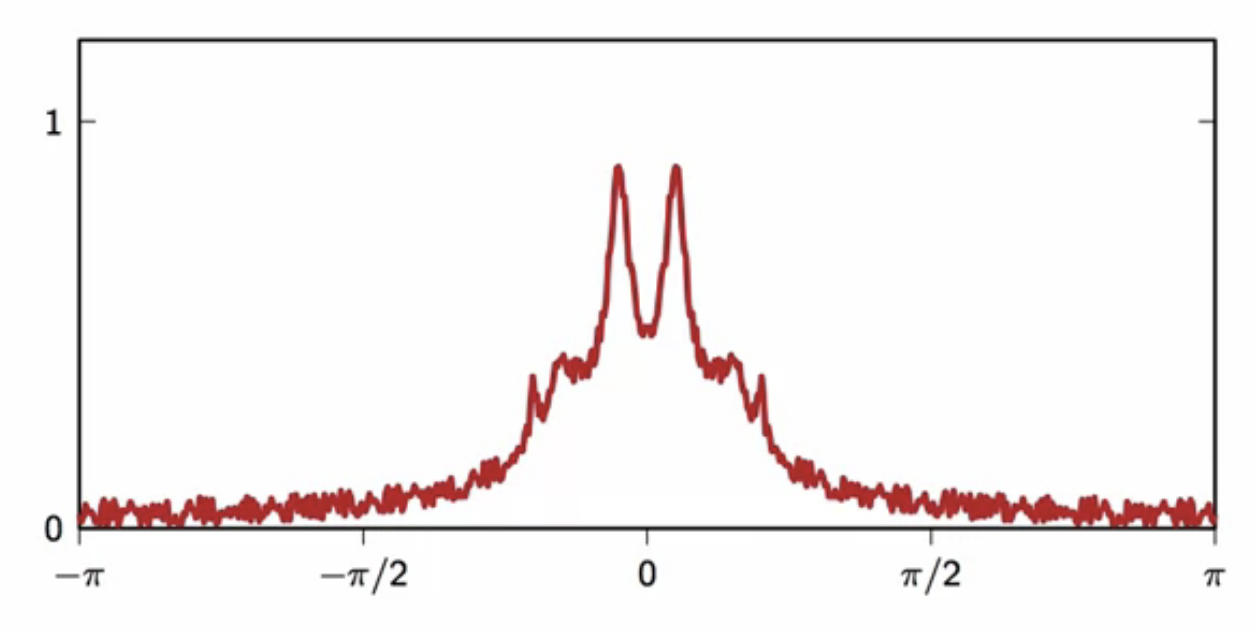
fig: frequency spectrum of noisy measured signal

phase analysis

• assume ( \vert H(e^{j \omega}) \vert = 1)
  • this is the phase of the filter frequency response
• there are three different phase analysis cases:
  • zero phase:
    • ( \angle H(e^{j \omega}) = 0)
    • spectrum is fully real
  • linear phase
    • ( \angle H(e^{j \omega}) = d\omega)
    • phase is proportional to the frequency
    • by a factor ( d \in mathbb{R})
  • non-linear phase
    • all other cases
• when a linear phase is added to a signal, its shape remains the same
  • it is shifted in time by the phase influenced amount
  • linear: phase is proportional to the frequency
• when a non-linear phase is added to a signal, its shape changes
  • non-linear: phase is not proportional to frequency
• the spectrum magnitude remains the same with phase changes

linear phase

• adding a phase is simply adding a delay to a signal \[ \begin{align} \mathcal{D} { x[n]} & = x[n - d]
  y[n] & = x[n-d]
  \end{align} ]
• in the frequency domain: [ \begin{align} Y( e^{j \omega}) & = e^{-j \omega d} X(e^{j \omega})
  H( e^{j \omega}) & = e^{-j \omega d} & \text{ phase }\propto \text{ } \omega \text{, by a factor of } d \end{align} ]
• the proportionality constant (d) in the frequency domain is the same as number of samples of delay by the delay operator in the time domain
  • this is why the phase change is linear
• this is also the reason why delay is inevitable in causal filters

---

moving-average filter

• the impulse response of the moving-average filter is \[ h[n] = (u[n] -u[n-M])/M ] fig: moving-average filter - impulse response

moving average - magnitude response

• the DTFT magnitude of the impulse response is \[ \vert He^{j\omega} \vert = \frac{1}{M} \Bigg \vert \frac{sin(\frac{\omega}{2}M)}{sin(\frac{\omega}{2})} \Bigg \vert ] - this magnitude is zero @ ( \omega = \frac{2\pi}{M} k ) when ( k \neq 0 ) fig: moving-average filter (M = 9) - impulse response DTFT (frequency response)

  fig: moving-average filter (M = 20) - frequency response

  fig: moving-average filter (M = 100) - frequency response

• in the frequency domain, when a moving-average filter is applied
  • this above noisy spectrum is multiplied with the frequency response of the moving-average filter

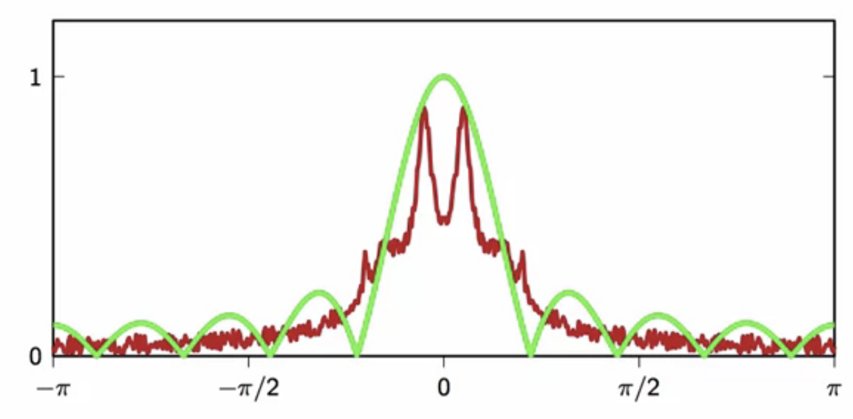
fig: noisy signal frequency spectrum overlaid with a 9-pt moving-average filter frequency spectrum

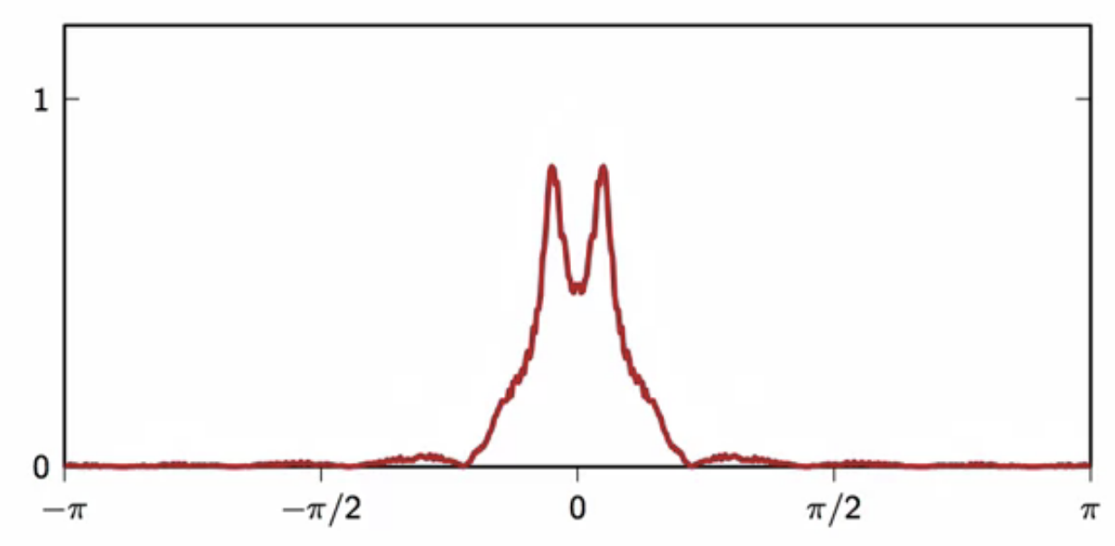
fig: product of noisy signal frequency spectrum with a 9-pt moving-average filter frequency spectrum

• this product indicates a high attenuation of high frequencies
• most of the noise contained in the high frequency band is eliminated

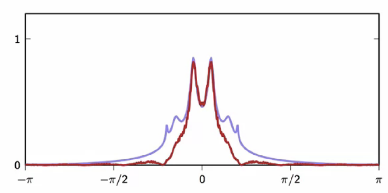
fig: original signal vs. filtered signal frequency spectrum

• some parts of the spectrum that carried useful information is also eliminated
• some useful information is lost in the process of removing noise

moving average - phase response

• moving average is a linear phase inducer
• moving-average filter frequency response including the phase is: \[ H( e^{j \omega}) = \frac{1}{M} \frac{sin(\frac{\omega}{2}M)}{sin(\frac{\omega}{2})} e^{-j \frac{M-1}{2} \omega} ]
  • here: [ \begin{align} \frac{1}{M} \frac{sin(\frac{\omega}{2}M)}{sin(\frac{\omega}{2})} & \text{: pure amplitude, real term}
    e^{-j \frac{M-1}{2} \omega} & \text{: pure phase term}
    d = \frac{M-1}{2} & \text{: half the length of the support in the impulse response}
    \end{align} ]
• half the length of the support in the impulse response is the delay introduced by the moving average

fig: moving-average filter response split into pure magnitude change, followed by pure phase change

[ \begin{align} H( e^{j \omega}) & = A(e^{j \omega})e^{-j \omega d}
A(e^{j \omega}) & \in \mathbb{R}
A(e^{j \omega}) & \text{: pure amplitude term}
e^{-j \omega d} & \text{: pure phase term}
\end{align} ]

---

leaky-integrator filter

• the impulse response of the leaky-integrator filter 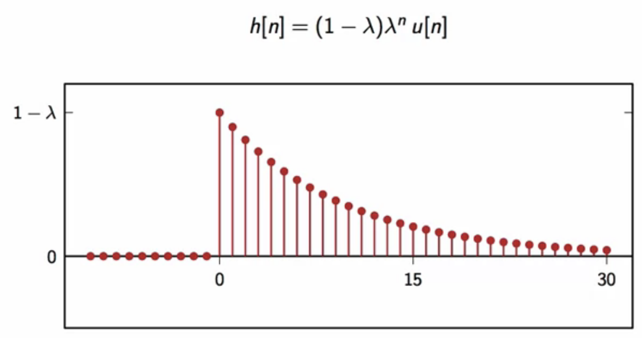fig: leaky-integrator impulse response
  • exponentially decaying sequence
• fourier-transform of leaky-integrator impulse response is
  \[ H( e^{j\omega} ) = \frac{1-\lambda}{1-\lambda e^{j\omega}} ]

complex algebra

[ \begin{align} \frac{1}{a + jb} & = \frac{a - jb}{a^2 + b^2}
\end{align} ]

• so, if [ \begin{align} x & = \frac{1}{a + jb}
  \end{align} ]
• then [ \begin{align} \vert x^2 \vert & = \frac{1}{a^2 + b^2} & \rightarrow \text{ magnitude }
  \angle x & = \tan^{-1} \Bigg [ -\frac{b}{a} \Bigg ] & \rightarrow \text{ phase }
  \end{align} ]

leaky integrator fourier transform

• consider the leaky integrator fourier transform [ \begin{align} H( e^{j\omega} ) & = \frac{1-\lambda}{1-\lambda e^{j\omega}}
  H( e^{j\omega} ) & = \frac{1-\lambda}{(1 - \lambda \cos \omega) - j \sin \omega}
  
  (1 - \lambda \cos \omega) & \rightarrow \text{ real part of denominator }
  \sin \omega & \rightarrow \text{ imaginary part of denominator }
  \end{align} ]
• applying complex algebra [ \begin{align} \vert H( e^{j\omega} ) \vert^2 & = \frac{(1-\lambda)^2}{1 - 2\lambda \cos \omega + \lambda^2} & \text{ squared magnitude }
  \angle H( e^{j\omega} ) & = \tan^{-1} \Bigg [ \frac{\lambda \sin \omega}{(1 - \lambda \cos \omega)} \Bigg ] & \text{ non-linear phase }
  \end{align} ]

leaky integrator - magnitude response

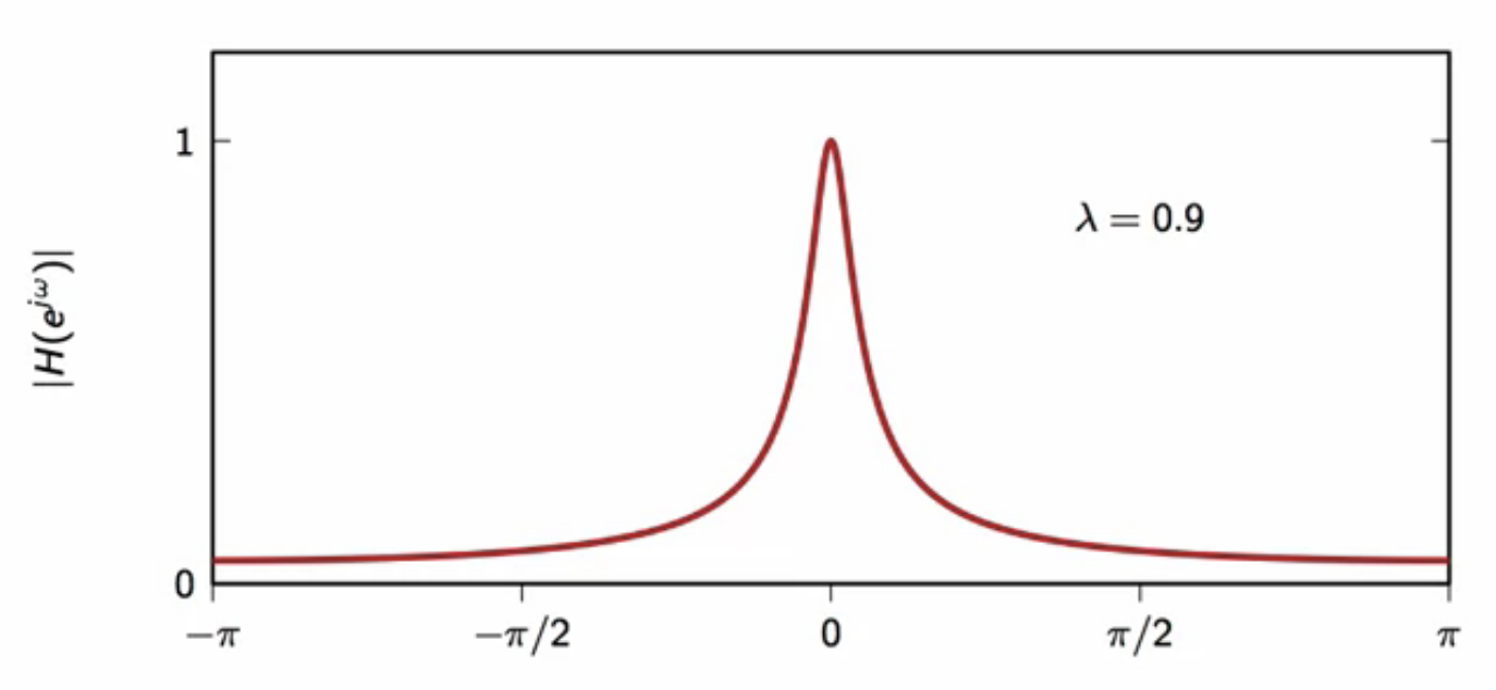
fig: leaky-integrator frequency response - magnitude (( \lambda = 0.9 ))

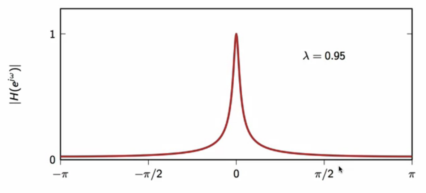
fig: leaky-integrator frequency response - magnitude (( \lambda = 0.95 ))

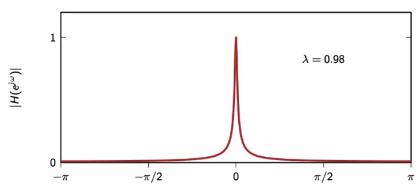
fig: leaky-integrator frequency response - magnitude (( \lambda = 0.98 ))

• characteristic is very similay to the moving average
  • however no zeros
  • monotonic and not oscilloscopic
• as (\lambda) goes closer to (1), the magnitude curve gets more concentrated around zero
  • becomes similar to the moving-average filter magnitude response when ( \lambda ) is very close ot (1)

leaky integrator - phase response

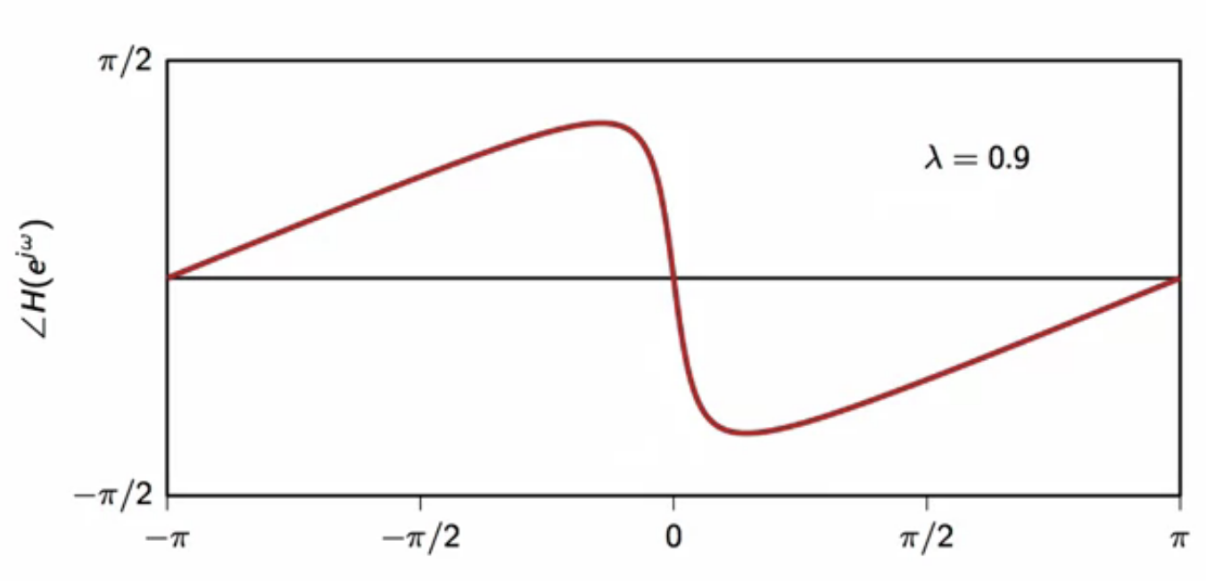
fig: leaky-integrator frequency response - phase (( \lambda = 0.9 ))

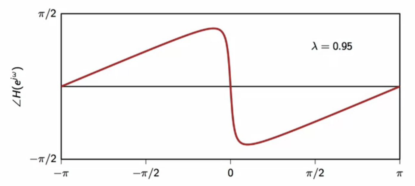
fig: leaky-integrator frequency response - phase (( \lambda = 0.95 ))

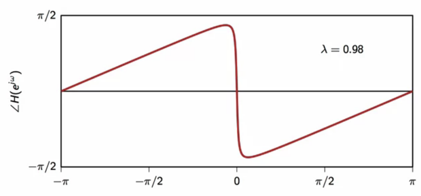
fig: leaky-integrator frequency response - phase (( \lambda = 0.98 ))

• non-linear characteristic
• as ( \lambda ) increases, the steepness of the phase curve increases

combined response

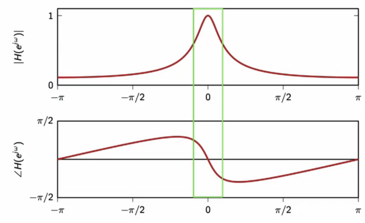
fig: linear part in the non-linear frequency response of a leaky integrator filter

• the part of the filter where the attenuation is not severe is linear
• so leaky integrator can be used without significant phase distortion

---

karplus-strong algorithm

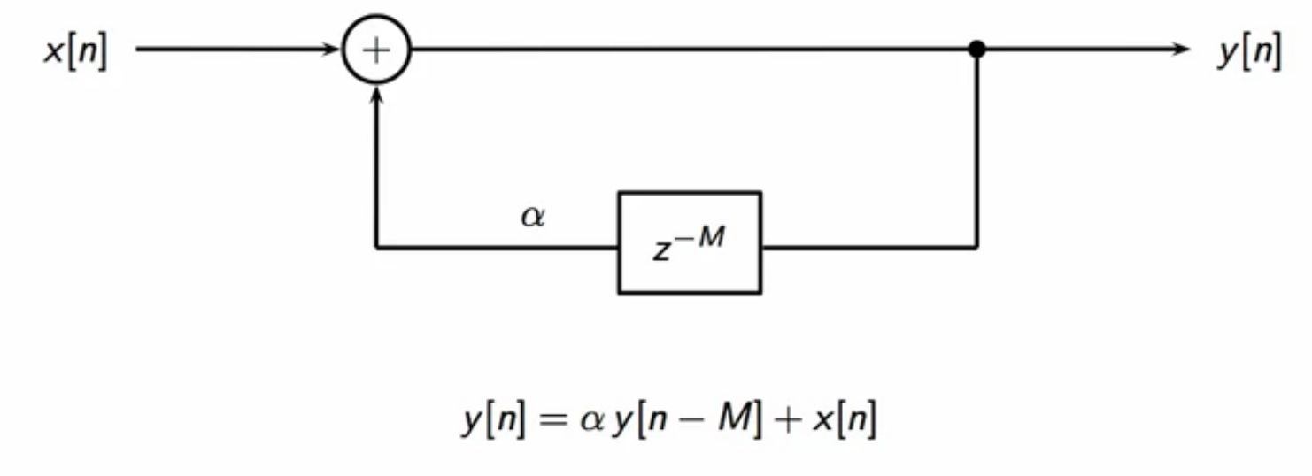
fig: karplus-strong signal generate algorithm

• this is initialized with a finite-support signal
• there is a feedback loop with a delay of (M) samples
  • feedback is scaled by a factor (\alpha)
• if Karplus-Strong algorithm is initialized with one period of the saw-tooth wave, then the following output is obtained
  • this is multiple repetitions of that period
  • with decay scaling influenced by (\alpha)

convolution in k-s algorithm

• consider a staggered exponential sequence \[ \begin{align} w[n] = \Bigg { \begin{matrix} \alpha^k & \text{ for } n = kM\ 0 & \text{ otherwise }\end{matrix}
  \end{align} ] - a series of exponentially decaying dirac-deltas - spaced (M) points apart
• the karplus-strong algorithm can be considered a convolution \[ \begin{align} y[n] & = \bar{x}[n] * w[n]
  \text{where: } &
  \bar{x}[n] &: \text{ finite-support signal used to initialize the k-s algorithm }
  w[n] &: \text{ a staggered exponential sequence }
  \end{align} ]
• the DTFT of this convolution gives [ \begin{align} Y( e^{j \omega} ) & = \bar{X}(e^{j \omega}) W(e^{j \omega})
  \bar{X} &: \text{ fourier transform of saw-tooth initialization signal }
  W(e^{j \omega}) &: \text{ fourier transform of staggered exponential sequence }
  \end{align} ]
• the DTFT of each component in the above equation is as follows: [ \begin{align} \bar{X} & = e^{ -j \omega } \Bigg ( \frac{M+1}{M-1} \Bigg ) \frac{ 1 - e^{-j(M-1)\omega} }{(1 - e^{ -j\omega })^2 } - \frac{1 - e^{-j(M + 1)\omega} }{(1 - e^{ -j\omega })^2}
  W(e^{j \omega}) & = \frac{1}{1 - \alpha e^{-j\omega M}}
  \end{align}

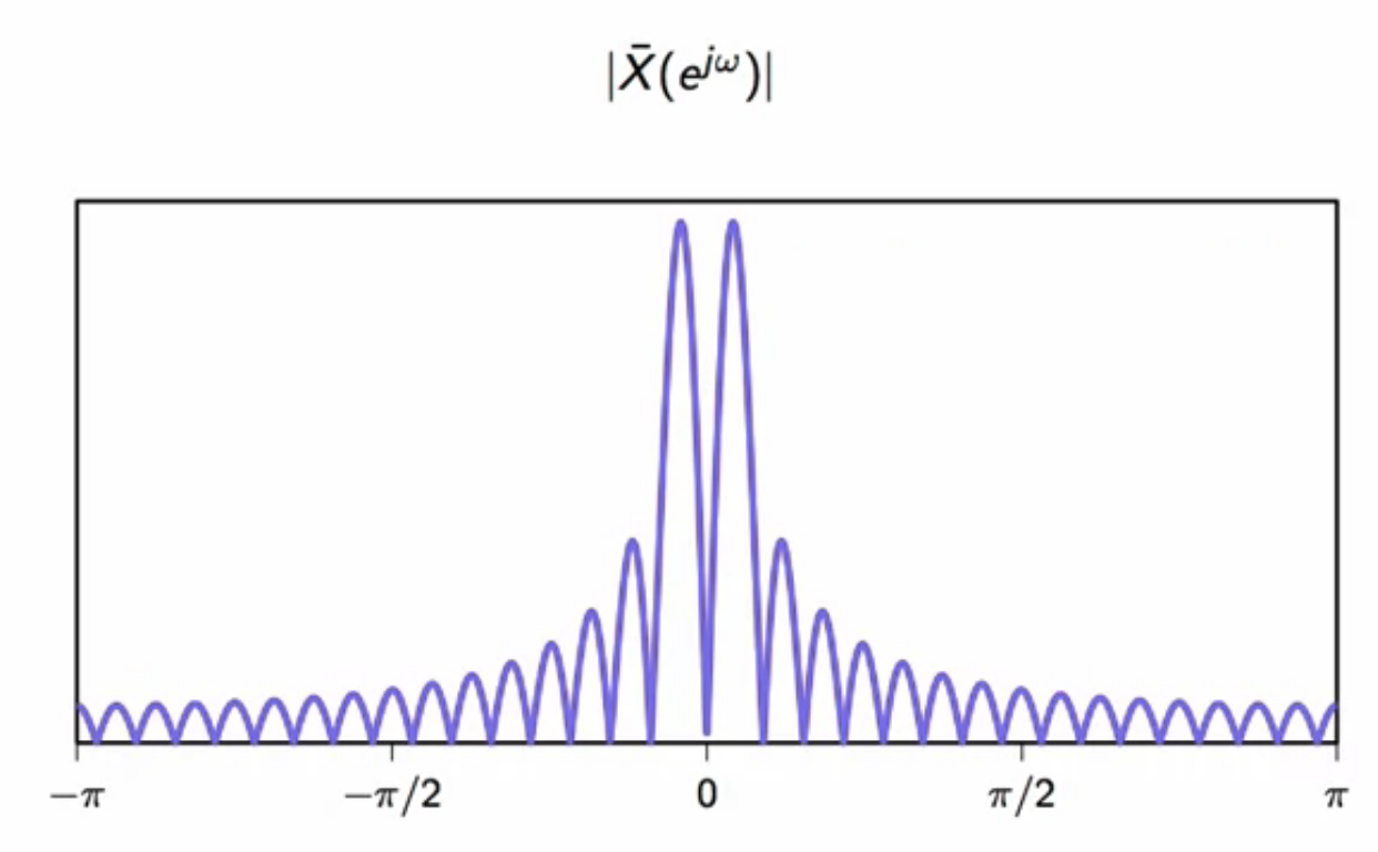
*fig: fourier transform of saw-tooth initialization wave*

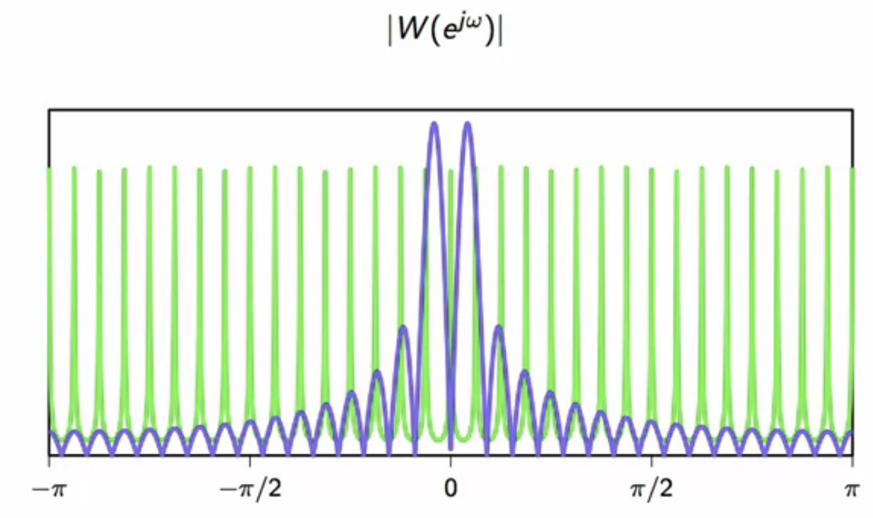
*fig: fourier transform of staggered exponential sequence overlaid on prev plot*

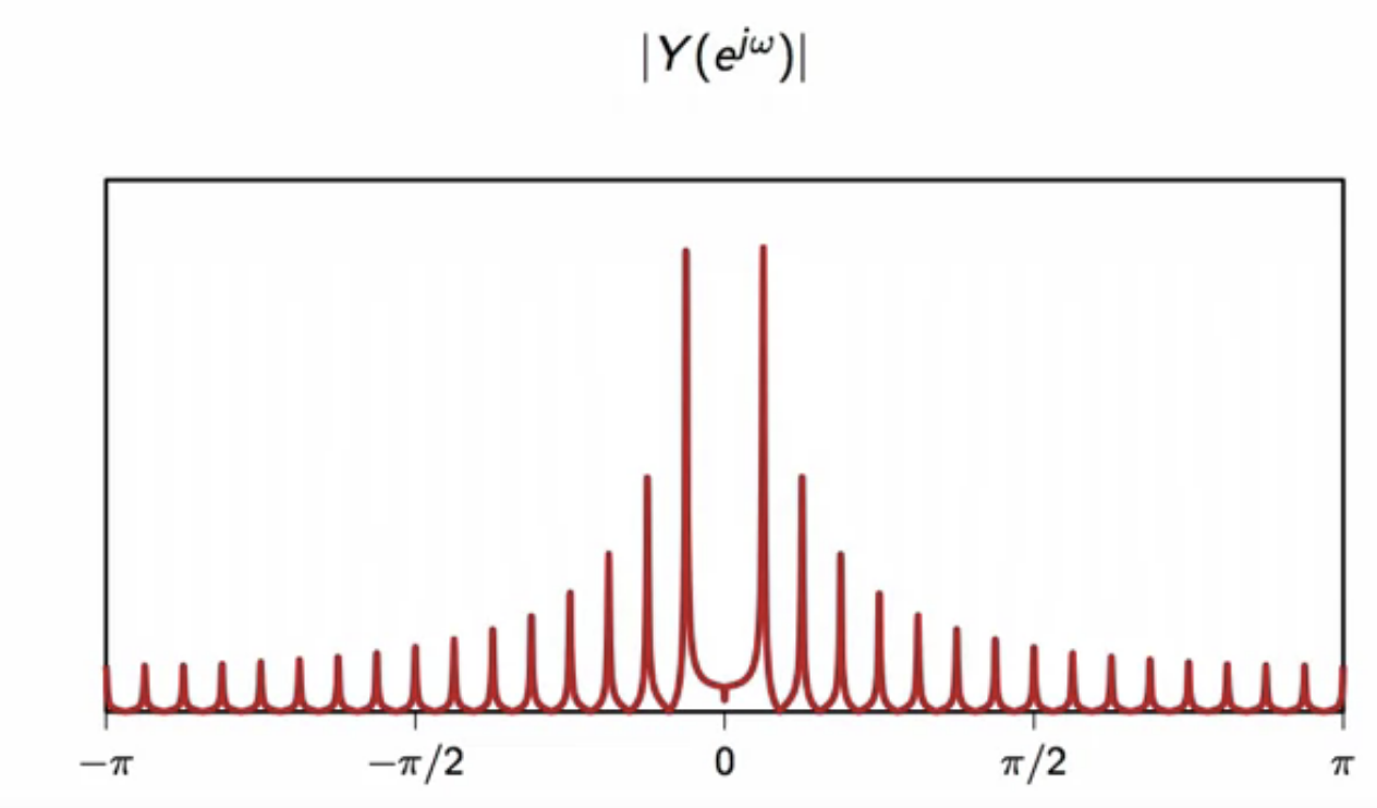
*fig: product of last two DTFT plots same as the karplus-strong fourier transform*

---

references

• ecole dsp - filters