[DSP] W06 - Designing Realizable Filters
contents
- CCDE
- CCDE frequency response
- existence and convergence
- rational transfer function
- stability criterion
- circus-tent method
- ideal filters cannot be implemented in real life
- constraints for a real filter:
- linearity
- time-invariance
- realizability
CCDE
CCDE represent causal LTI systems
- CCDE: Constant Coefficient Differential Equation
- a linear combination of past input and output values
- scaled by constants
[ \sum_{k=0}^{N-1} a_k y[n-k] = \sum_{k=0}^{M-1} b_k x[n-k] ]
- uses (M) inputs and (N) outputs
- MIMO: Multiple Input Multiple Output systems
- LTI systems can only contain
- additions
- delays
- multiplications by constant (scaling)
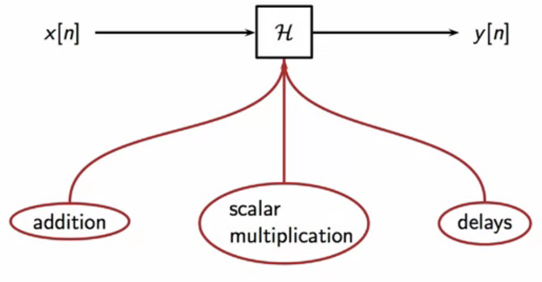
fig: SISO LTI filter requirements
- a causal LTI system’s output is a linear function of past values of the input and output
CCDE frequency response
- (z)-transform is a tool to find the frequency response of the system equation
- is a power series
- maps a discrete time sequence (x[n]) to a function of the complex variable (z)
- formally, the (z)-transform is given by \[ X(z) = \sum_{n = -\infty}^{\infty} x[n]z^{-n}, \text{ } z \in \mathbb{C} ]
- (z)-transform is a generalization of the DTFT for points in the whole complex plane - the (z)-transform of (x[n]) at (z = e^{j\omega}) is the same as the DTFT of (x[n]) \[ X(z)\vert_{z=e^{jw}} = DTFT { x[n] } ]
properties of the (z)-transform
- linearity \[ \mathcal{Z}{ \alpha x[n] + \beta y[n] } = \alpha X(z) + \beta Y(z) ]
- time-shift \[ \mathcal{Z} { x[n-N] } = z^{-N} X(z) ]
application to CCDE
- using the linearity and time-shift properties, the following relationship is obtained
[ \begin{align}
\sum_{k=0}^{N-1} a_k y[n-k] & = \sum_{k=0}^{M-1} b_k x[n-k] & \rightarrow \text{CCDE} _
_
_Y(z) \sum{k=0}^{N-1} a_k z^{-k} & = X(z) \sum_{k=0}^{M-1} b_k z^{-k} & \rightarrow z\text{-transform}
Y(z) & = H(z)X(z)
\end{align}
]
- here, the (z)-transform of the output is the product of the (z)-transform of the input with a function (H(z)) [ H(z) = \frac{\sum_{k=0}^{M-1} b_k z^{-k}}{\sum_{k=0}^{N-1} a_k z^{-k}} ]
- (H(z)) is the ratio of two polynomials in variable (z)
- the coefficients of the polynomials are the coefficients that appear in the CCDE
- in the numerator: coefficients of CCDE input (b_k)
- in the denominator: coefficients of CCDE output (a_k)
- to get frequency response of system defined by CCDE, set (z = e^{j\omega})
[ \begin{align}
H(z) & = H(e^{j\omega})
Y(e^{j\omega}) & = H(e^{j\omega}) X(e^{j\omega}) \end{align} ] - this is in the form of the relationship between the input and output of a filtering operation
- so (H) is a filter
- (H)’s frequency response is computed by the polynomial ratio obtained by the frequency response
existence and convergence
- each case the (z)-transform is applied to has a Region Of Convergence (ROC)
- ROC determines points on the complex plane where the (z)-transform exists
- existence of the (z)-transform is the same as the convergence of the power series that defines the transform
- ROC is where the power series can converge
- since (z)-transform is a power series, when it converges, it converges absolutely
- i.e. convergence depends only on the magnitude of (z), not on its phase
- absolute convergence condition \[ \vert X(z) \vert < \infty \Leftrightarrow \sum_{n = -\infty}^{\infty} \vert x[n] z^{-n} \vert < \infty ]
three cases of ROC
- (z)-transform of finite-support sequence
- the transform is the sum of a finite number of terms
- so convergence is guaranteed
- in other cases, the ROC of the (z)-transform has circular symmetry
- depends only only on (\vert z \vert)
- if it converges on one point of the complex plane, it converges on all points with the same magnitude
- this is a circle on the complex plane
- ROC for causal sequences
- extends from a circle to infinity
- ROC extends outside a circle on the complex plane,
- not inside the circle
rational transfer function
- in the (z) domain, a CCDE is represented as (H(z)), which is the ratio of tw polynomials of (z^{-1})
- this polynomial is called a rational transfer function
- an LTI transfer function:
[ H(z) = \frac{ b_0 + b_1 z^{-1} + \ldots + b_{M-1} z^{M-1} }{a_0 + a_1 z^{-1} + \ldots + a_{N-1} z^{N-1}}
]
- ratio of polynomials
- polynomial of degree (M-1) in numerator
- polynomial of degree (N-1) in denominator
- the frequency response of a filter is equal to this transfer function evaluated at (z = e^{j\omega} )
- transfer function can also be expressed as
[ H(z) = C \frac{\prod_{n=1}^{M-1} (1 - z_n z^{-1}) }{\prod_{n=1}^{N-1} (1 - p_n z^{-1}) }
]
- ( z_n ): zeros of the transfer function
- roots of the first order terms in the numerator
- they send the transfer function to zero
- represented by filled up ‘O’ in the complex plane
- ( p_n ): poles of the transfer function
- roots of the first order terms in the denominator
- send the denominator to zero
- so they are trouble spots for ROC
- represented by ‘X’ in the complex plane
- ( z_n ): zeros of the transfer function
- this transfer function is analyzed for the ROC of the system defined by the transfer function
causal system ROC
- for a causal system, we know that the ROC
- extends outwards from a circle
- cannot include poles
- zeros do not affect the region of convergence
- so ROC extends outwards from a circle touching the largest-magnitude poles
- this circle size is determined by the poles
- the circle can touch the pole but not have it in the ROC
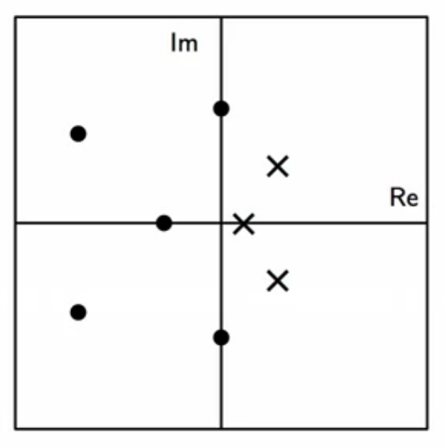
fig: plot of zeros and poles of a causal system in the complex plane
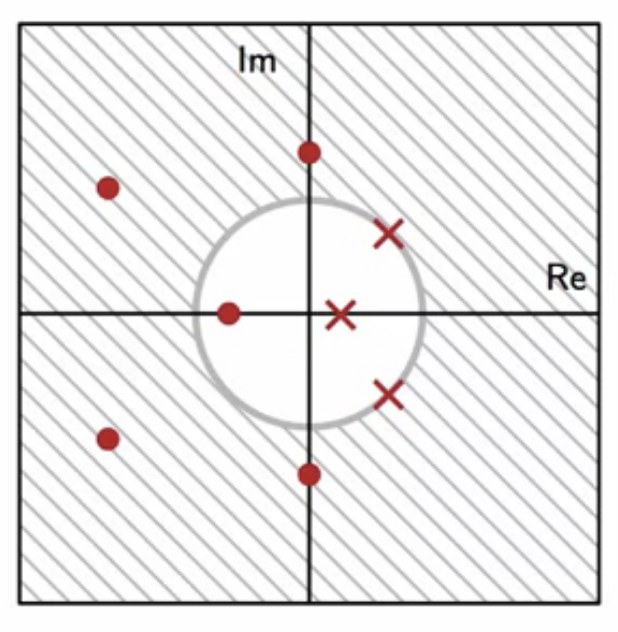
fig: circle and shaded area indicates ROC for a causal system
stability criterion
- the ROC definition obtained from the poles of transfer function helps defines the stability of the system
- a stability criterion which depends on knowing the transfer function of the system can be defined
- the necessary and sufficient condition for BIBO stability is impulse response must be absolutely summable \[ \sum_{n=-\infty}{\infty} \vert h[n] \vert < \infty ]
- absolute convergence property of (z)-transform
- when (z)-transform exists for (\vert z \vert = 1)
- (z)-transform converges absolutely
- this implies that the impulse response is absolutely summable
- conversely, if impulse response is absolutely summable
- it is implied that (z)-transform converges absolutely, and
- (z)-transform exists for (\vert z \vert = 1)
- so, the stability criterion for a system is
- the ROC includes the unit circle
“system is stable only if its ROC contains the unit circle”
- this means that all the poles of the transfer function must be inside the unit circle
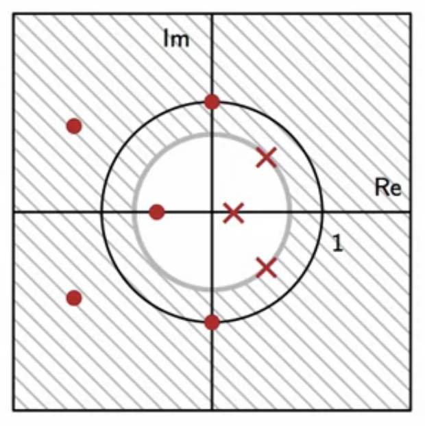
fig: stable system - poles inside unit circle, ROC contains the unit circle
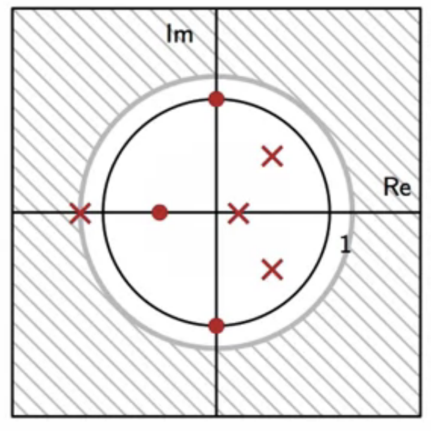
fig: unstable system - poles outside unit circle, unit circle not in ROC
circus-tent method
- this is a method to estimate frequency response of a system from the complex plane pole-zero plot
procedure
- assume that the magnitude of the (z)-transform is like a rubber sheet over the complex plane
- this sheet glued to the ground at the zeros of the transfer function
- the poles push the rubber sheet up
- frequency response in magnitude is the profile of the sheet around the unit circle
example
- consider the following pole-zero plot
- has two zeros and two poles
- complex poles always exist in pairs as complex conjugates
- this true for all real valid systems
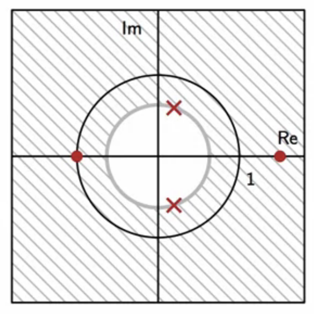
fig: circus tent method - stable system ROC, includes unit circle
- consider the complex plane in a 3D perspective
- the horizontal plane in the complex plane
- the height is the magnitude of the frequency response (H(z))of the transfer function
- assume ( H(z) = 1 ) as the starting point for the rubber sheet
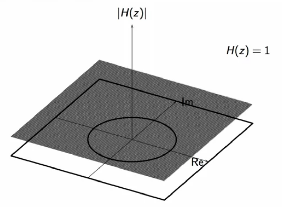
fig: circus tent method - 3D perspective of frequency response of transfer function
- estimation process:
- glue the rubber sheet to the complex plane where the zeros are fig: circus tent method - frequency response glued to ground at zeros
- poles at poles push the sheet to infinity fig: circus tent method - poles pushing the frequency response fabric
- this is the shape of the rubber sheet having considered all four components on the complex plane
- the fourier transform is the value of the (z)-transform around the unit circle
- this is the level curve of the rubber sheet computed along the unit circle
fig: circus tent method - level curve on fabric along unit circle
- this is the level curve of the rubber sheet computed along the unit circle
- plotting this level circle in ( [-\pi,\pi] ) fig: circus tent method - frequency response obtained by spreading out level curve in ( [-\pi,\pi] )
- the circus-tent method provides understanding about the relationship between
- the frequency response and
- the zero-pole plot obtained from the system transfer function