[DSP] W07 - Interpolation

contents

• polynomial interpolation
  • interpolation requirements
  • polynomial interpolation
  • lagrange interpolation
• local interpolation
  • zero-order interpolation
  • first-order interpolation
  • third-order interpolation
• local interpolations schemes
  • three kernels
• sinc interpolation
  • example
  • lagrange-sinc interpolation relationship
• trade-offs

---

• interpolation is the process of synthesizing continuous-time world entities from the discrete-time world
• symbolically, $x\left(t\right)$ is obtained, given $x\left[n\right]$

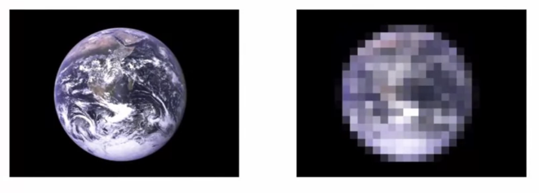
fig: continuous-time world vs. discrete-time world metaphor

---

polynomial interpolation

• consider given a discrete sequence of points

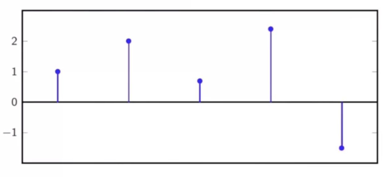
fig: discrete time sequence

• to be determined is a continuous function that goes through all the points

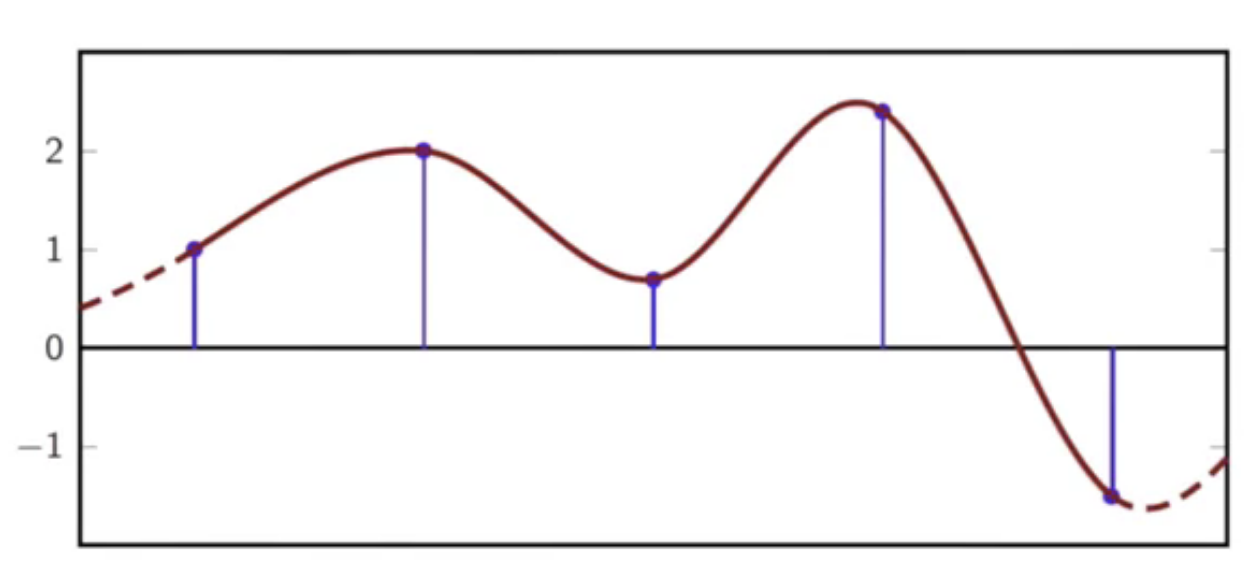
fig: continuous curve fit through discrete time sequence

• this transforms $x\left(t\right)$ to $x\left[n\right]$
• interpolators are tools to generate curves through points in a localized area
  • these are used to generate band-limited continuous-time functions

interpolation requirements

• decide on $T_s$: spacing between the samples
• make sure $x\left(n{T}_s\right)=x\left[n\right]$
• $x\left(t\right)$ has to be smooth

smoothness entailment

• smoothness means:
  • the interpolation should be infinitely differentiable
• jumps (1st order discontinuities) requires signals to move faster than light

• 2nd order discontinuities requires infinite acceleration

• natural solution: polynomial interpolation

polynomial interpolation

• this is a naive approach for the interpolation problem
• for a discrete signal with $N$ points
  • polynomial of degree $N-1$
• fit the polynomial
  • $p\left(t\right)=a_0+a_{1}t+a_2{t}^2+\dots +a_{N-1}{t}^{N-1}$
• here: $$\begin{array}{ccccc}p\left(0\right)& =x\left[0\right]p\left(T_s\right)& =x\left[1\right]p\left(2T_s\right)& =x\left[2\right]\dots p\left(\right(N-1\left)T_s\right)& =x[N-1]\end{array}$$

lagrange interpolation

• consider a symmetric interval $I_N=[-N,\dots ,N]$
• set $T_s=1$

• then: $$\begin{array}{ccccc}p(-N)& =x[-N]p(-N+1)& =x[-N+1]\dots p\left(0\right)& =x\left[0\right]\dots p\left(N\right)& =x\left[N\right]\end{array}$$

• $P_N$: space of degree-$2N$ polynomials over $I_N$

• a basis for $P_N$ is the family of $2N+1$ lagrange polynomials $$L_n^{\left(N\right)}\left(t\right)=\prod _{k=-N,k\ne n}^N\frac{t-k}{n-k}n=-N,\dots ,N$$

• pick N = 1 to get three lagrange polynomials
  • $L_{-1}^{\left(1\right)},L_0^{\left(1\right)},L_1^{\left(1\right)}$

• calculate each polynomial now:

• $L_0^{\left(1\right)}$:
  • ${\prod }_{k=-1}^1\frac{t-k}{-k}=\frac{t+1}{1}.\frac{t-1}{-1}=1-t^2$
  • this is a parabola
    • which is 1 at origin
    • 0 at 1 and -1
• similarly,
  • $L_1^{\left(1\right)}\left(t\right)=\frac{t^2+t}{2}$
  • $L_{-1}^{\left(1\right)}\left(t\right)=\frac{t^2-t}{2}$

• all lagrangian polynomials generated so are 1 at their index $N$ and 0 at other integers

• lagrangian interpolator: $$p\left(t\right)=\sum _{n=-N}^{N}x\left[n\right]L_n^{\left(N\right)}\left(t\right)$$

• this interpolation is the sough-after polynomial interpolator
• polynomial of degree $2N$ through $2N+1$ points in unique
• the lagrangian interpolator satisfies $$p\left(n\right)=x\left[n\right]\text{for}-N\le n\le N\text{since}{L}_n^{\left(N\right)}\left(m\right)=\{\begin{array}{cc}1& \text{if}n=m\\ 0& \text{if}n\ne m\end{array}$$

example

• given sequence

fig: discrete time sequence

• the lagrange interpolation with $N=2$ is as follows
  • this has five lagrange polynomials in all: $L_{-2}^{\left(2\right)},L_{-1}^{\left(2\right)},L_0^{\left(2\right)},L_1^{\left(2\right)},L_2^{\left(2\right)}$

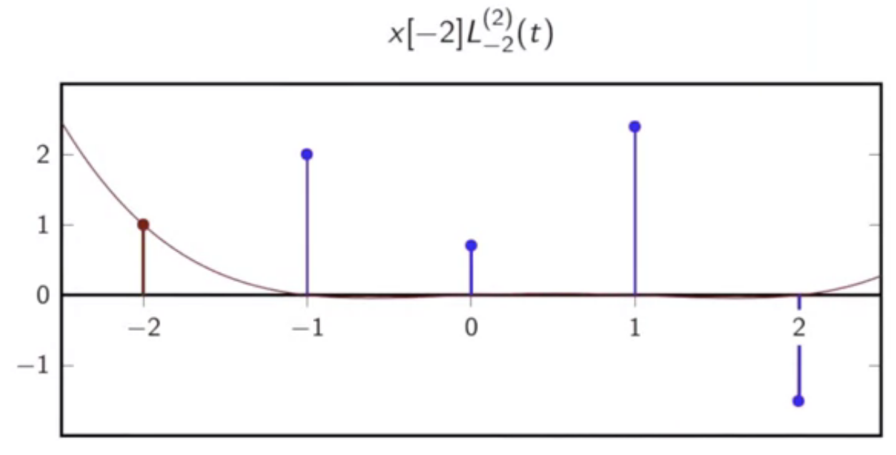
fig: lagrange polynomial [-2]

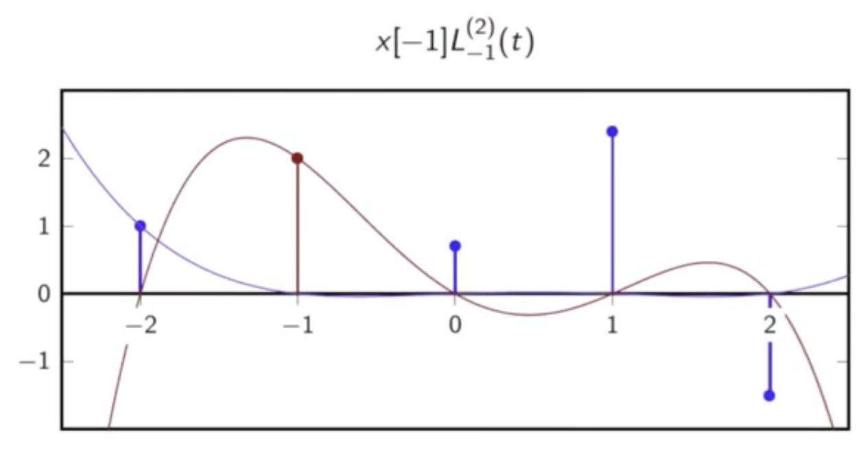
fig: lagrange polynomial [-1]

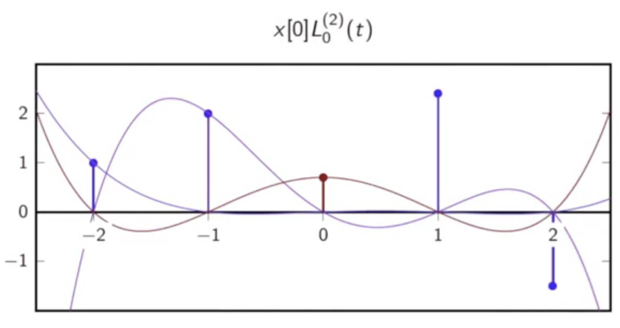
fig: lagrange polynomial [0]

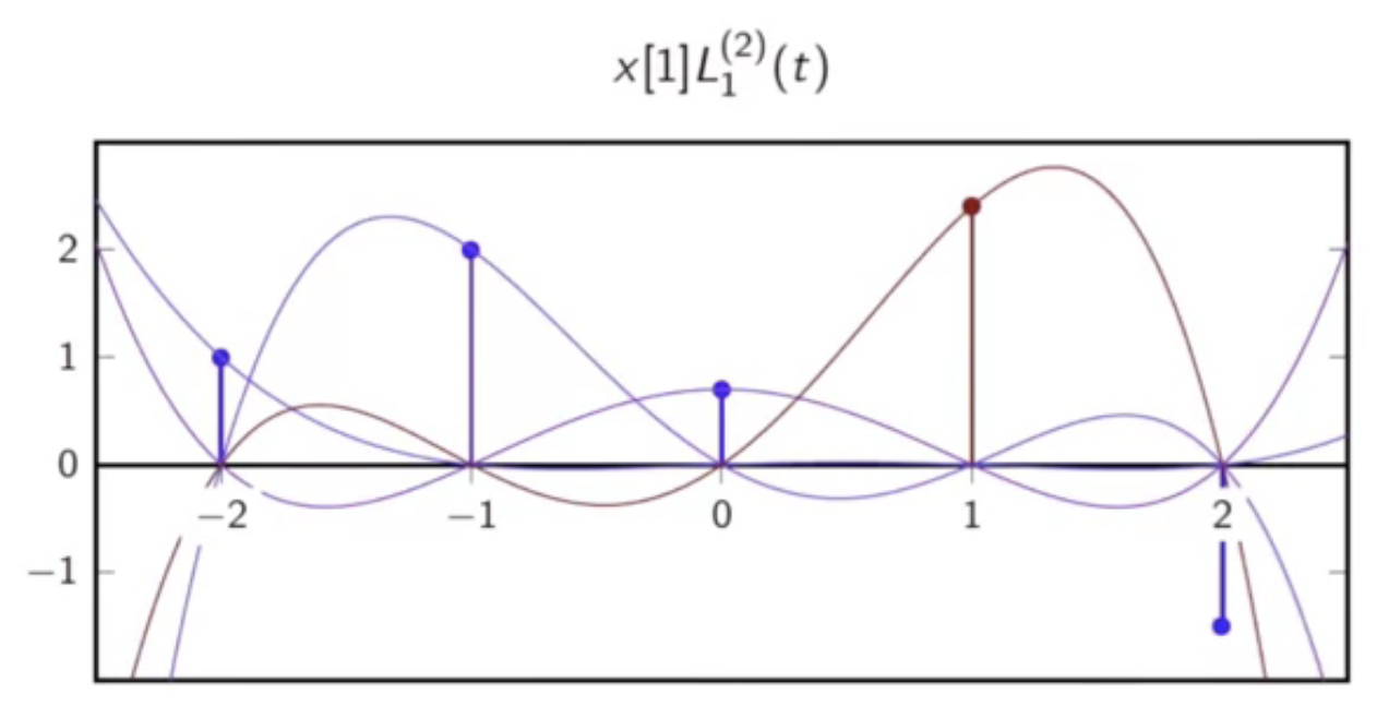
fig: lagrange polynomial [1]

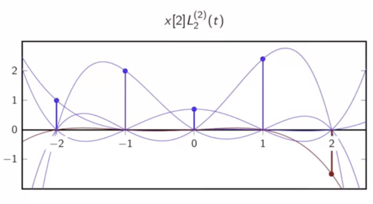
fig: lagrange polynomial [2]

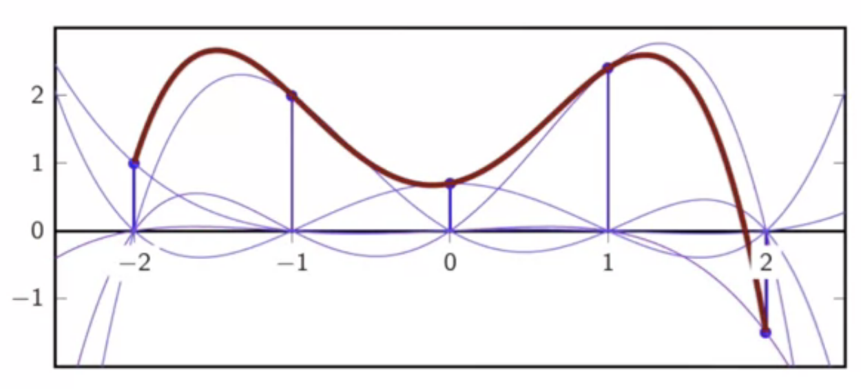
fig: summed lagrange polynomials

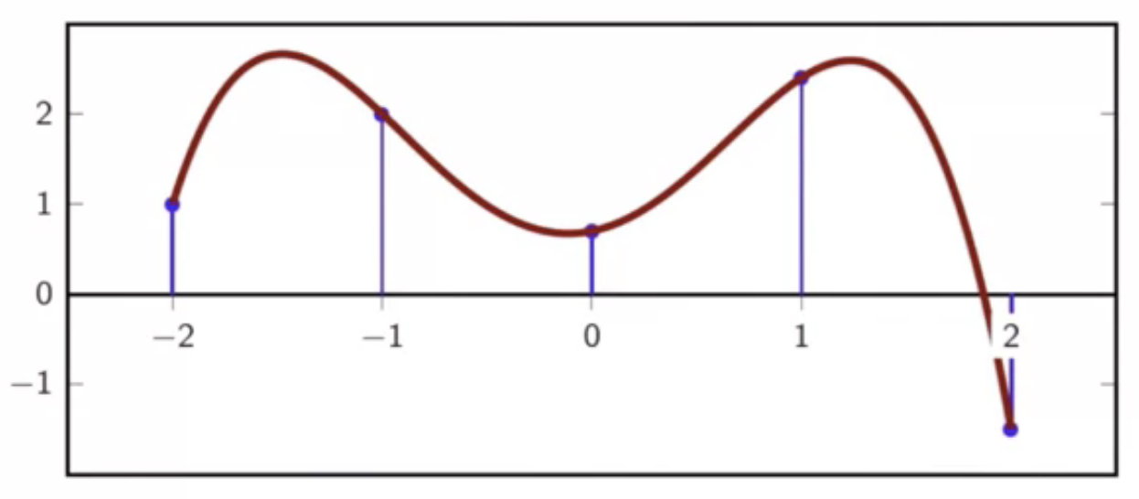
fig: final interpolation to given discrete signal

lagrange polynomial notes

• maximally smooth

• infinitely many continuous derivatives

• interpolation bricks shape depend on chosen $N$
• each brick looks different

---

local interpolation

• other interpolation possibilities essentially have to meet the same requirements
  • decide on $T_s$
  • make sure $x\left(n{T}_s\right)=x\left[n\right]$
  • $x\left(t\right)$ has to be smooth
• smoothness condition of being infinitely many times differential is too stringent for practical applications

• signal has to hold smoothness within the limits of the system

• consider the following sequence in discrete-time

fig: discrete time sequence

• explored in the following are some interpolation strategies

zero-order interpolation

• piecewise constant function
  • a staircase function
• matches discrete sequence value at given locations
• but is not continuous

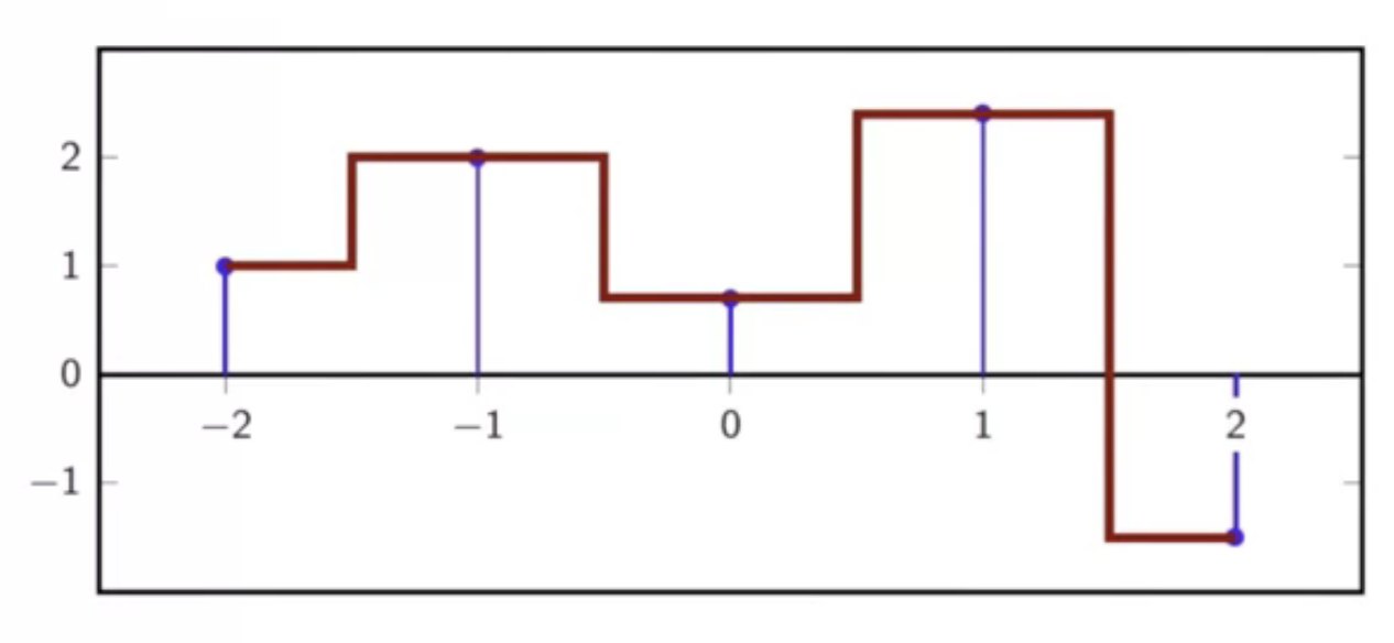
fig: piecewise interpolation for a discrete time sequence

characteristics

• $x\left(t\right)=x[\lfloor t+0.5\rfloor ]$
  • $-N\le t\le N$

$$x\left(t\right)=\sum _{n=-N}^{N}x\left[n\right]rect(t-n)$$

• interpolation kernel: $i_0\left(t\right)=rect\left(t\right)$
• $i_0\left(t\right)$: “zero-order hold”
  • interpolator’s support is 1
  • interpolation is not continuous

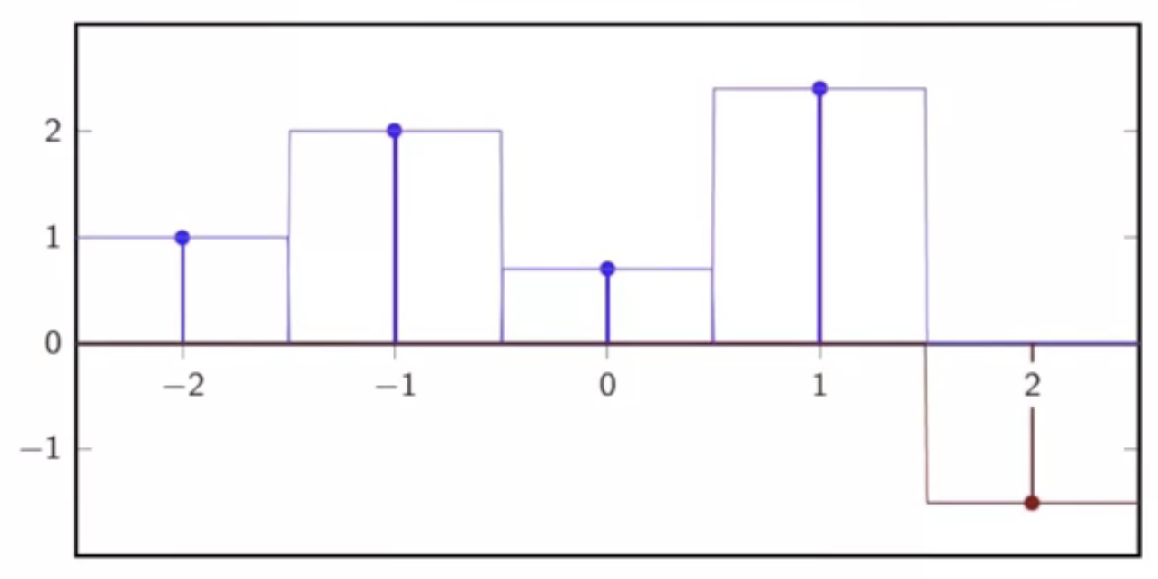
fig: zero-order interpolation - rects for a discrete time sequence

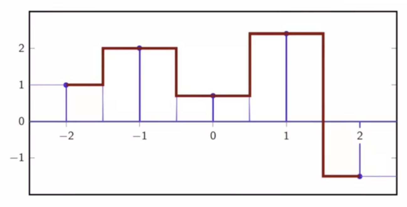
fig: sum of piecewise rect supports

first-order interpolation

• piece-wise linear function

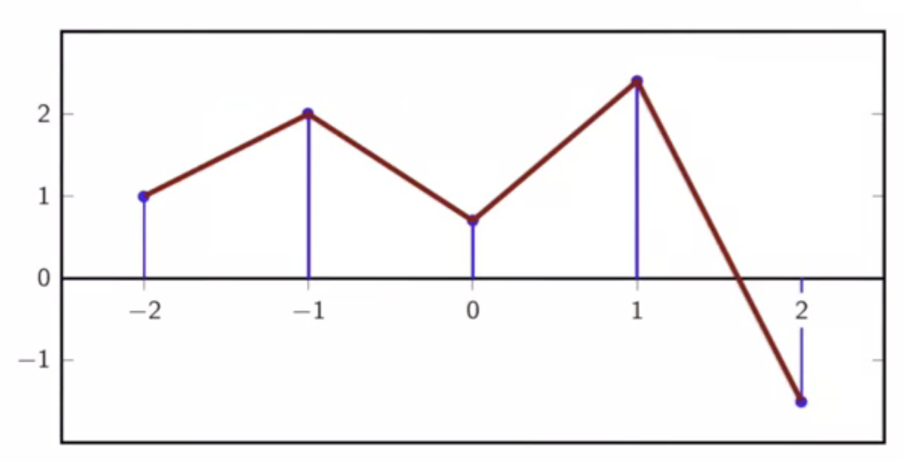
fig: first-order interpolation for a discrete time sequence

• straight lines connect the samples
• connect the dots strategy

characteristics

$$x\left(t\right)=\sum _{n=-N}^{N}x\left[n\right]i_1(t-n)$$

• interpolation kernel: $$i_1\left(t\right)=\{\begin{array}{cc}1-\left|t\right|& \left|t\right|\le 1\\ 0& \text{otherwise}\end{array}$$
• interpolator support is 2
• interpolation is continuous
  • however its derivative is not
• the interpolation function has inflections at the discrete sample points

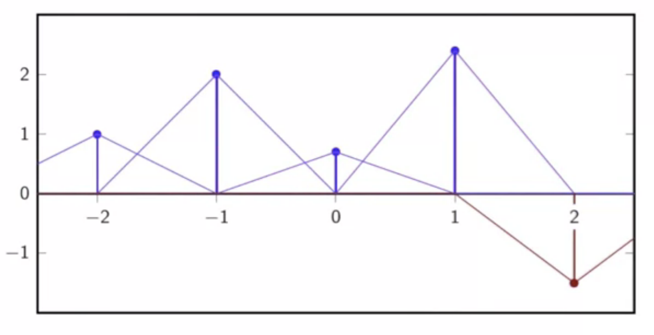
fig: first-order interpolation - support functions through discrete sequence

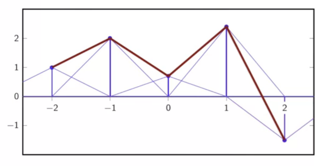
fig: first-order interpolation - sum of support functions

third-order interpolation

characteristics

$$x\left(t\right)=\sum _{n=-N}^{N}x\left[n\right]i_3(t-n)$$

• interpolation kernel is put together from two cubic polynomials
• interpolator support is 4
• interpolation is continuous up to second derivative

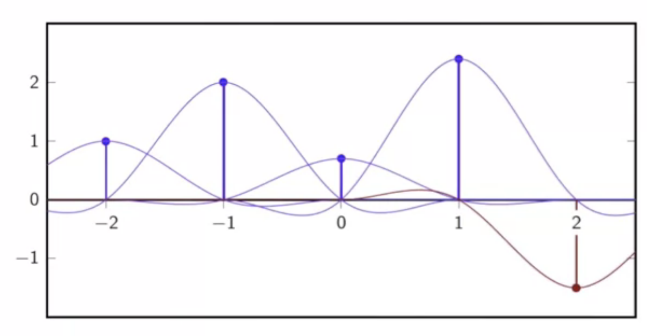
fig: third-order interpolation - support functions through discrete sequence

fig: third-order interpolation - sum of support functions

---

local interpolations schemes

$$x\left(t\right)=\sum _{n=-N}^{N}x\left[n\right]i_c(t-n)$$

• interpolator’s requirements:
  • $i_c\left(0\right)=1$
  • $i_c\left(t\right)=$ for $t$ a nonzero integer
• different interpolator kernels may be used with the interpolator

three kernels

• box kernel

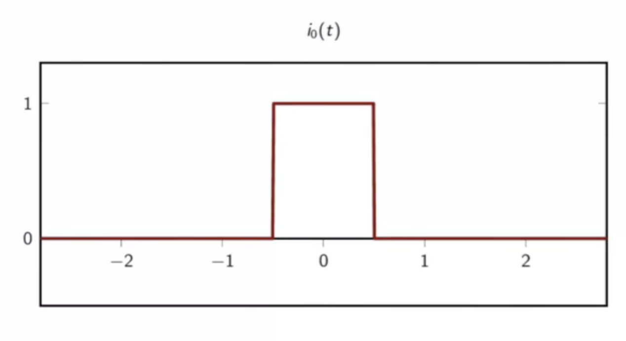
fig: box interpolator kernel

• triangle kernel

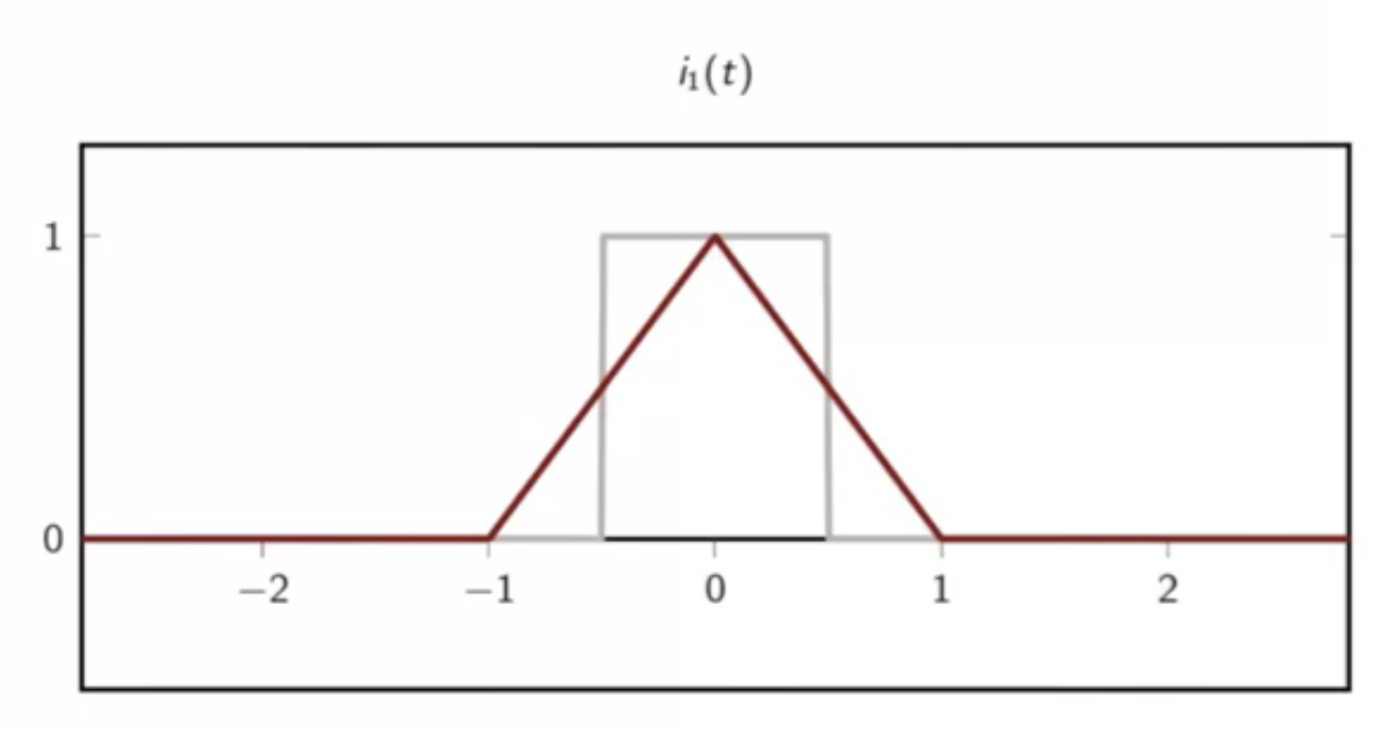
fig: triangle interpolator kernel

• cubic kernel

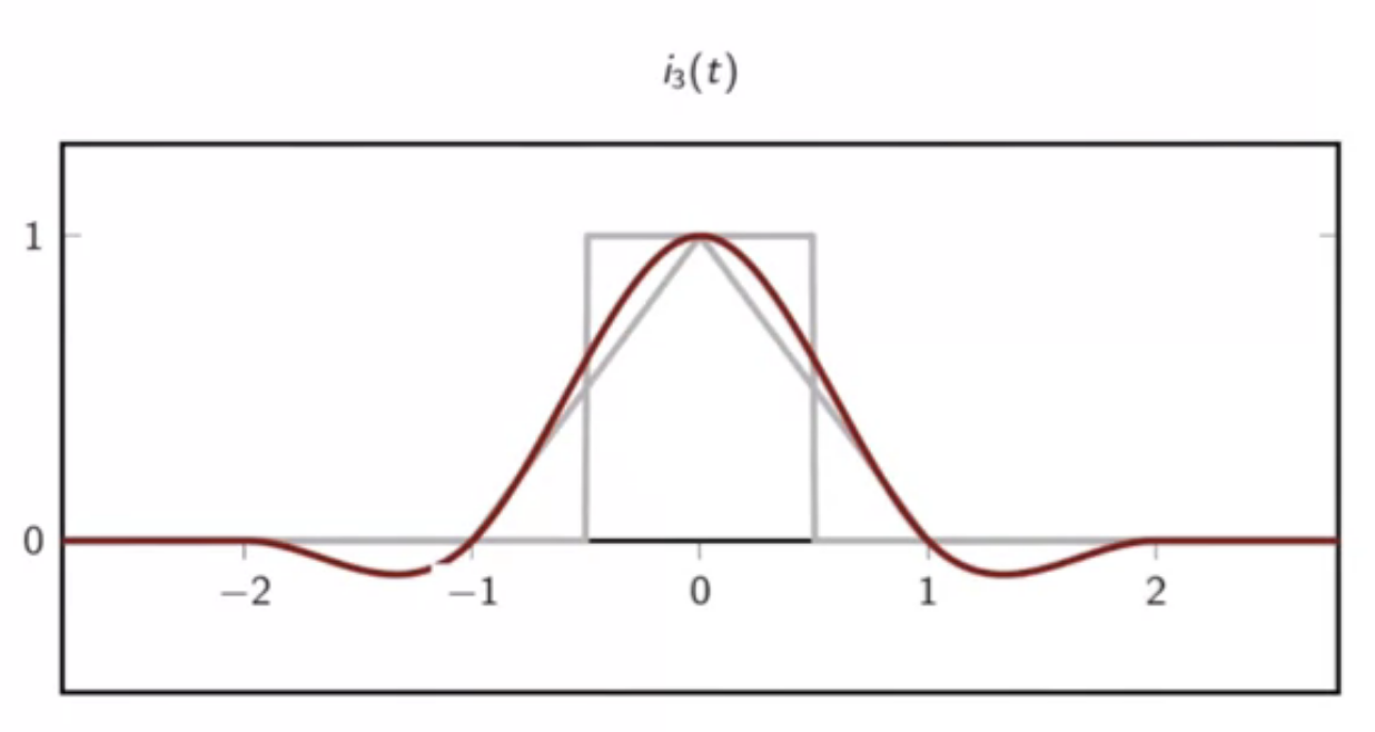
fig: cubic interpolator kernel

properties

• they become larger and smoother as the order increases
• same interpolating function independent of $N$
  • in contrast with the lagrange interpolation
• lack of smoothness
  • compared to the lagrange interpolation

---

sinc interpolation

$$x\left(t\right)=\sum _{n=-\infty }^{\infty }x\left[n\right]sinc(\frac{t-n{T}_s}{T_s})$$

example

• consider a discrete-time sequence

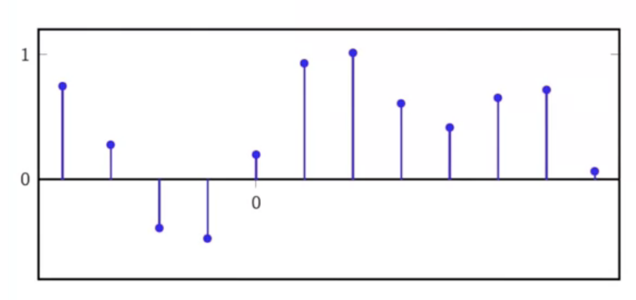
fig: discrete-time sequence to be interpolated

• overlaying the interpolator kernels over appropriate sequence points

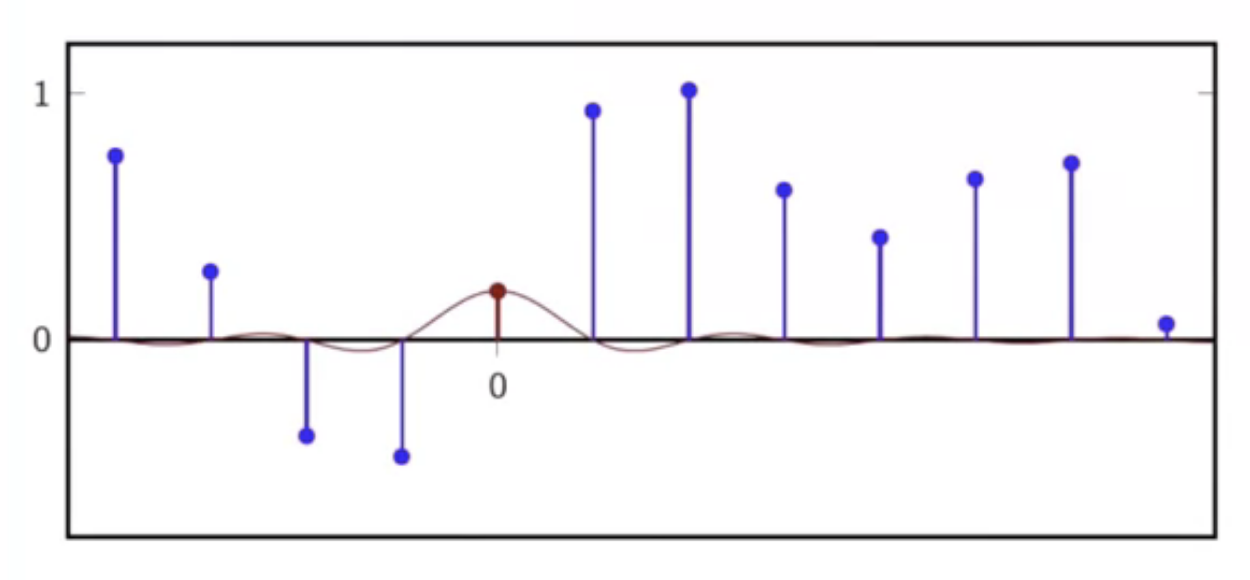
fig: one kernel, at origin

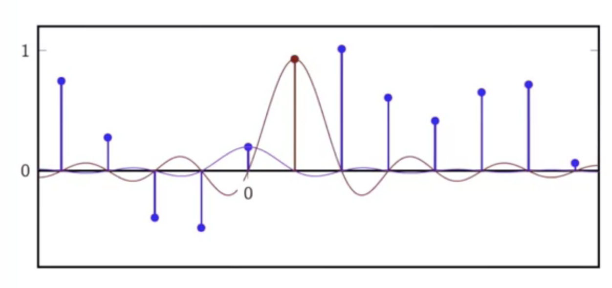
fig: second kernel added

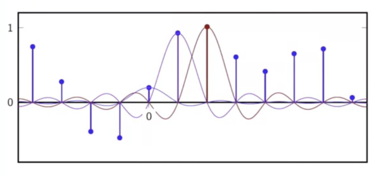
fig: more kernels added

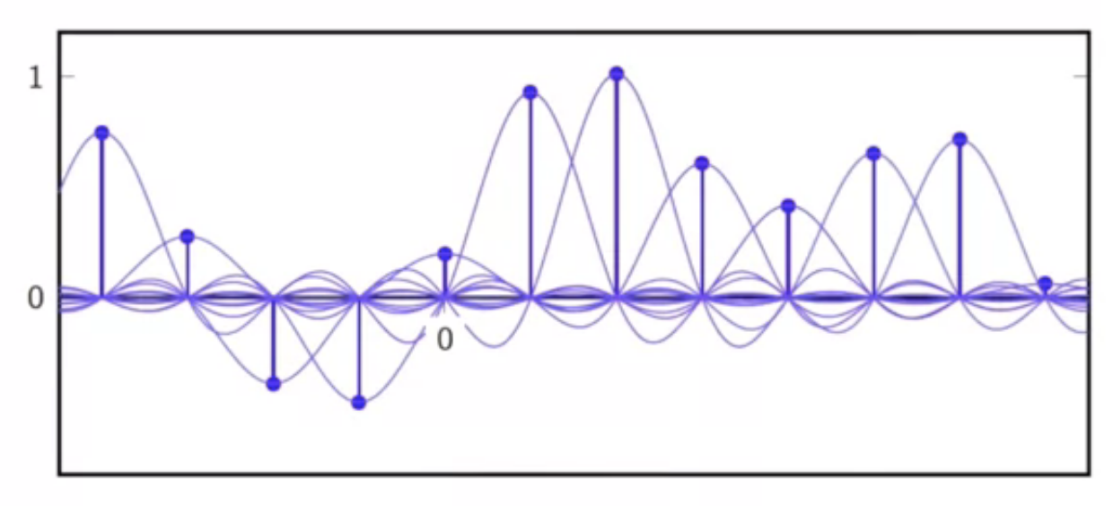
fig: all discrete samples fitted with corresponding kernels

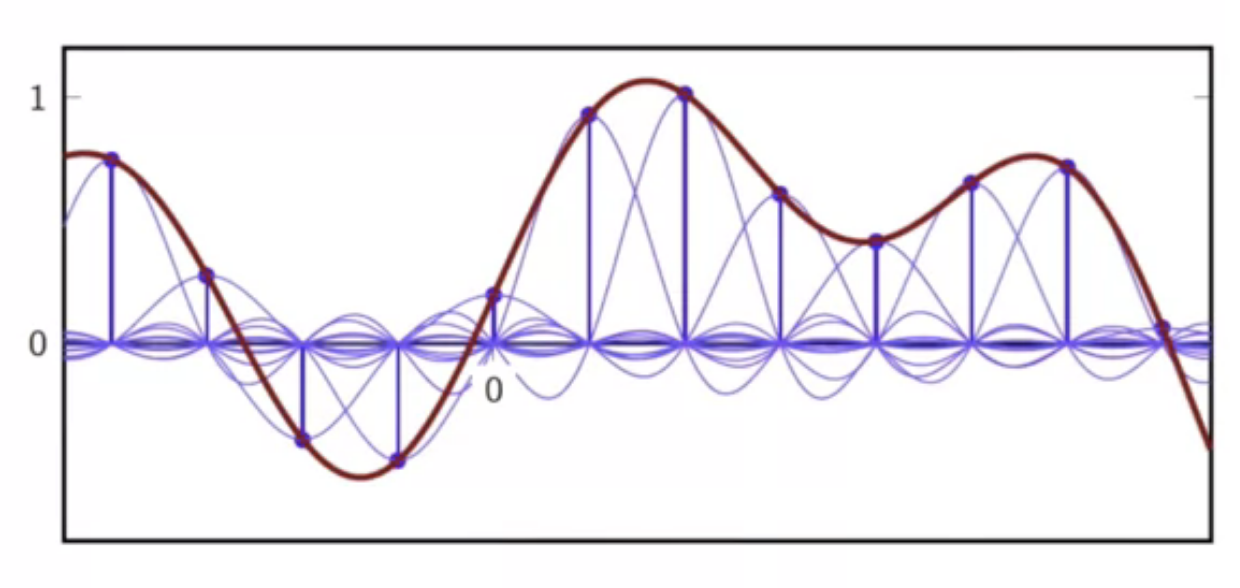
fig: sum of support kernels

lagrange-sinc interpolation relationship

• lagrange-sinc interpolation relationship $$\underset{N\to \infty }{lim}{L}_n^{\left(N\right)}=sinc(t-n)$$
• within the system limit, local and global interpolation are the same
  • lagrange interpolation: global
  • sinc interpolation: local

proof

• proof is too technical (see textbook)
• intuition: $sinc(t-n)$ and $L_n^{\left(\infty \right)}\left(t\right)$ share infinite number of zeros

$$\begin{array}{cccc}sinc(m-n)& =\delta [m-n]& & \\ & m,n\in Z{L}_n^{\left(N\right)}\left(m\right)& =\delta [m-n]& m,n\in Z,\\ & -N\le n,m\le N& & \end{array}$$

visualization

• below are comparisons of sinc and higher order lagrange function interpolation

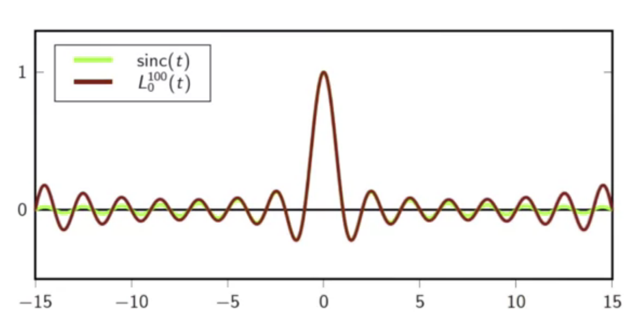
fig: sinc and 100-order lagrange interpolator

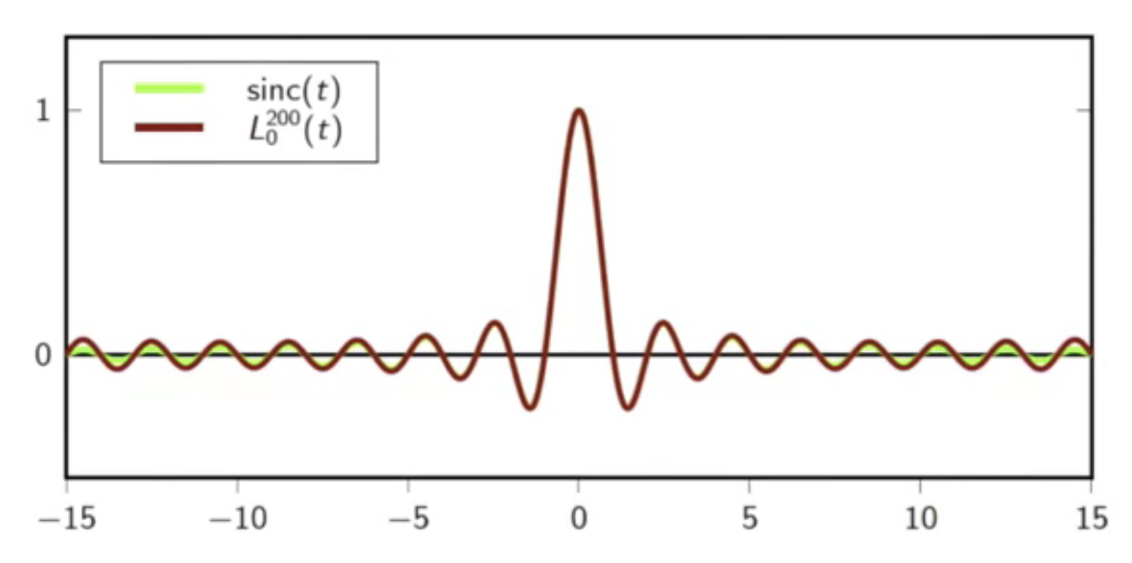
fig: sinc and 200-order lagrange interpolator

fig: sinc and 300-order lagrange interpolator

---

trade-offs

• lagrange interpolation is maximally smooth
  • but has the drawback that the interpolation kernel depends on N.
• to avoid lagrange interpolation drawback, another interpolation called local interpolation is used
  • method uses only a neighborhood of 2N+1 points and
  • an interpolation kernel over these 2N+1 points that is equal to 1 at zero and 0 at nonzero integer points

• the interpolation kernel does not depends on N but some of the smoothness is lost in the process

• as N goes to infinity, the lagrange interpolation corresponds to a sinc interpolation
  • at the limit, global and local interpolation are equivalent

---

references

• ecole dsp - filters