[DSP] W07 - Sampling Bandlimited Functions
contents
- sinc interpolation
- fourier transform of interpolated function
- space of bandlimited functions
- sampling theorem
- references
- when an arbitrary sequence is interpolated with the sinc interpolator, the result is necessarily a bandlimited function
- bandlimited functions belongs to a subspace (of bandlimited functions)
- sampling theorem works only in this subspace
- bandlimited function may be reconstructed perfectly by sampling them uniformly-spaced in this space
sinc interpolation
\[ x(t) = \sum_{n = -\infty}^{\infty} x[n] sinc \bigg( \frac{t - nT_s}{T_s} \bigg) ]
- input:
- discrete-time signal (x[n]), ( n \in \mathbb{Z} )
- (DTFT{ x[n] = X(e^{j\omega})} )
- interpolation interval: (T_s)
- the sinc function
- output:
- a smooth, continuous-time signal ( x(t), \text{ } t \in \mathbb{R} )
sinc relationships
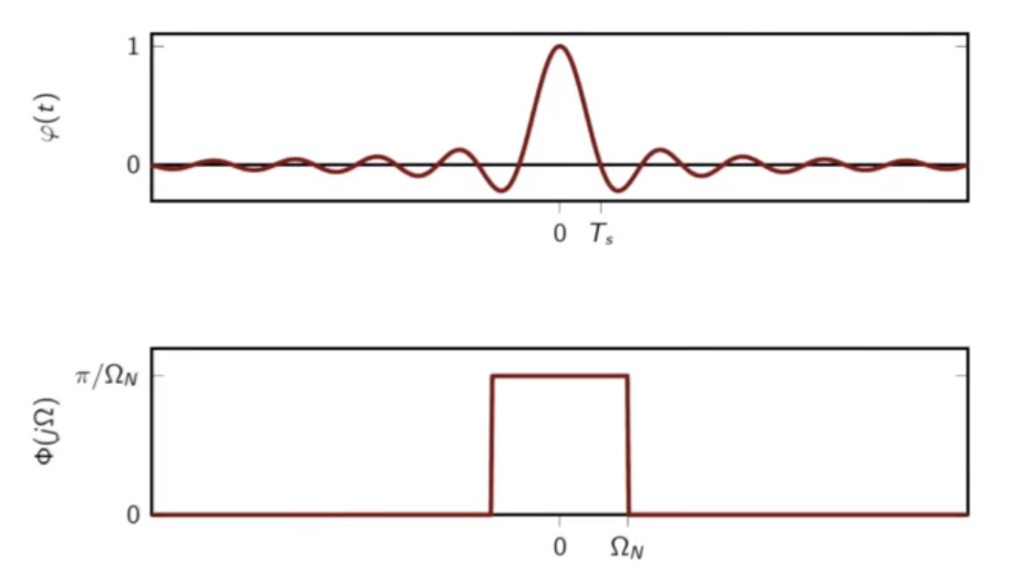
[ \varphi(t) = sinc \bigg( \frac{t}{T_s} \bigg)
T_s = \frac{\pi}{\Omega_N}
\text{ fourier-transform of } \varphi(t)
\Phi(j\Omega) = \frac{\pi}{\Omega_N} rect \bigg( \frac{\Omega}{2 \Omega_N} \bigg)
\Omega_N = \frac{\pi}{T_s}
]

fig: sinc kernel and its fourier transform
fourier transform of interpolated function
- the sinc function is given by
\[ x(t) = \sum_{n = -\infty}^{\infty} x[n] sinc \bigg( \frac{t - nT_s}{T_s} \bigg) ]
- the CTFT is computed on this equation
[ \begin{align}
X(j\Omega) & = \int_{-\infty}^{\infty} x(t) e^{-j\Omega t} dt _
& = \int{-\infty}^{\infty} \sum_{n = -\infty}^{\infty} x[n] sinc \bigg( \frac{t - nT_s}{T_s} \bigg) e^{-j\Omega t} dt _
& = \sum{n = -\infty}^{\infty} x[n] \int_{-\infty}^{\infty} sinc \bigg( \frac{t - nT_s}{T_s} \bigg) e^{-j\Omega t} dt _
& = \sum{n = -\infty}^{\infty} x[n] \bigg( \frac{\pi}{\Omega_N} \bigg) rect \bigg( \frac{\Omega}{2\Omega_N} \bigg) e^{-j n T_s \Omega}
\end{align}
]
interpolation CTFT analysis
[
\begin{align}
X(j\Omega) & = \sum_{n = -\infty}^{\infty} x[n] \bigg( \frac{\pi}{\Omega_N} \bigg) rect \bigg( \frac{\Omega}{2\Omega_N} \bigg) e^{-j n T_s \Omega} _
& = \bigg( \frac{\pi}{\Omega_N} \bigg) rect \bigg( \frac{\Omega}{2\Omega_N} \bigg) \sum{n = -\infty}^{\infty} x[n] e^{-j (\frac{\pi}{\Omega_N}) \Omega_n}
& = \Bigg { \begin{matrix} \big( \frac{\pi}{\Omega_N} \big) X(e^{j\pi(\frac{\Omega}{\Omega-N})}) & \text{ for } \vert \Omega \vert \leq \Omega_N \ 0 & \text{ otherwise }\end{matrix}
\end{align}
]
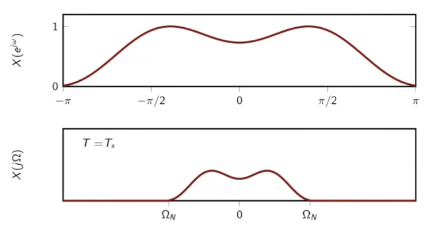
comparing DTFT and CTFT

fig: DTFT of (x[n]) and CTFT of ( x(t) ) - comparison
- same shape but rescaled
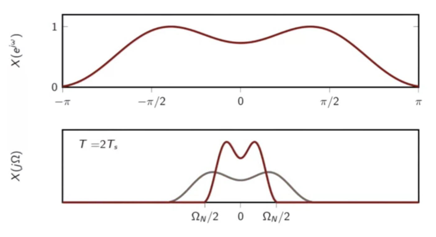
- when sampling interval is doubled
- the spectrum is contracted and sharpened

fig: comparing DTFT of (x[n]) and CTFT of ( x(t) ) - sampling doubled
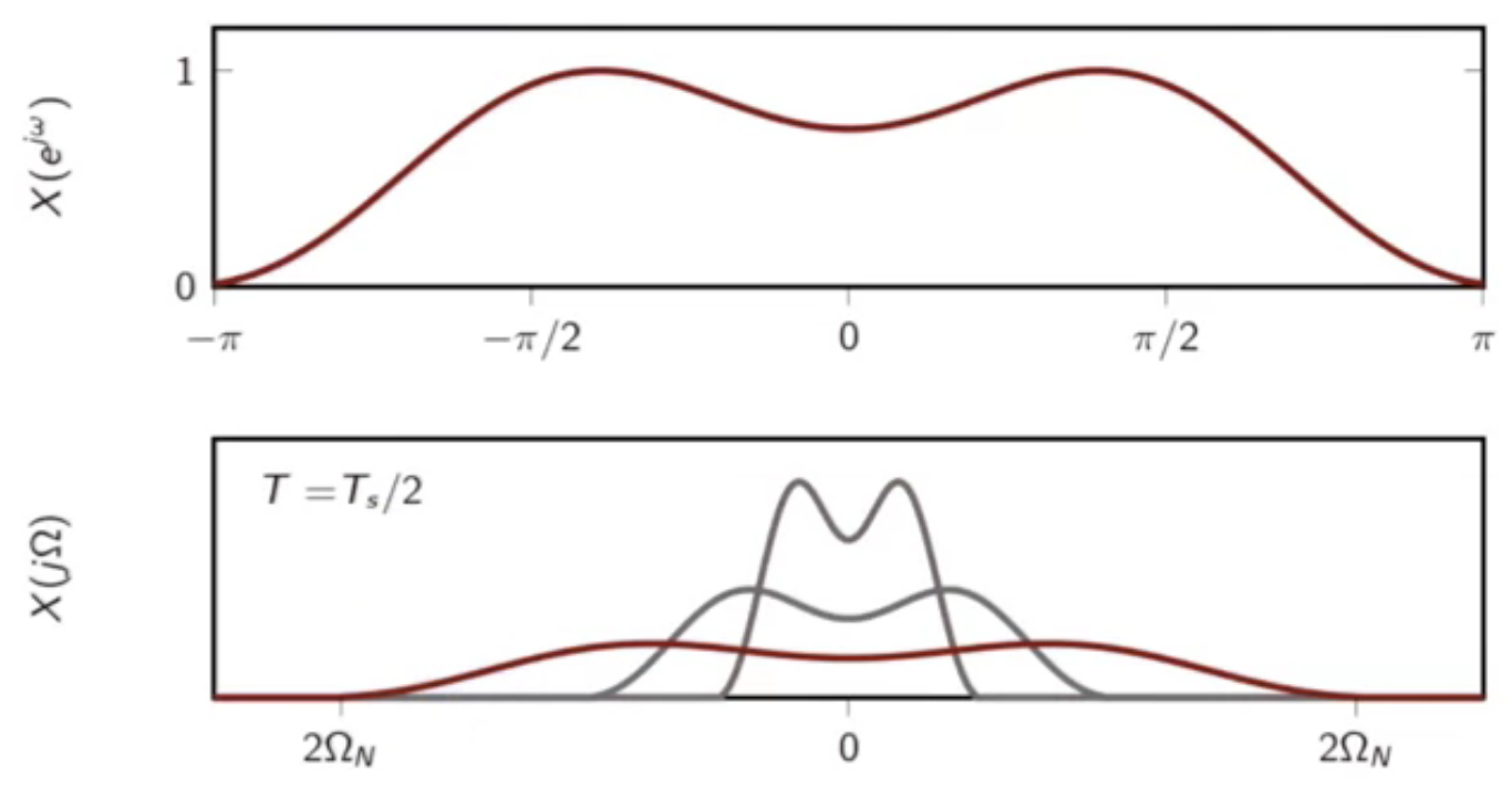
- when sampling interval is halved
- the spectrum is expanded and flattened

fig: comparing DTFT of (x[n]) and CTFT of ( x(t) ) - sampling halved
sampling interval
- if samples are closer together, the signal becomes faster
- if samples are further apart, the signal is slower
- pick interpolation period (T_s)
- (X(j\Omega)) is (\Omega_N)-bandlimited
- ( \Omega_N = \frac{\pi}{T_s} )
- fast interpolation ((T_s) small ) (\rightarrow ) wider spectrum
- slow interpolation ((T_s) large ) (\rightarrow ) narrower spectrum
- (X(j\Omega)) is (\Omega_N)-bandlimited
space of bandlimited functions
- after interpolation, assumption is
- (x[n]) is uniquely represented by (x(t))
- interpolation mapping: \[ x[n] \in \ell_2(\mathbb{Z}) \overset{T_s}{\longrightarrow} \begin{matrix} x(t) \in L_2(\mathbb{R}) \ \Omega_N-BL \end{matrix} ]
- the sampling theorem states that the original sequence used to interpolate a signal may be obtained by sampling the interpolated signal
assumptions
- assume (T_s = 1 ) and ( \Omega_N = \pi )
- the space of ( \Omega_N = \pi ) bandlimited funtions is a Hilbert space
- the functions ( \varphi^{(n)}(t) = sinc(t-n)), with ( n \in \mathbb{Z} ), form a basis for this space
- if (x(t)) is (\pi-BL), the sequence (x[n] = x(n) ) with ( n \in \mathbb{Z} )
- this is a sufficient representation
- i.e. (x(t)) may be reconstructed from (x[n])
- this is the essence of the sampling theorem
space of (\pi-BL) functions
- this is vector space
- because (\pi-BL \subset L_2(\mathbb{R}) )
- linear combinations of (\pi-BL) functions are (\pi-BL) functions
- inner product is standard inner product in (L_2(\mathbb{R})) [ \langle x(t), y(t) \rangle = \int_{-\infty}^{\infty} x^*(t)y(t) dt ]
- convolution [ (x y)(t) = \langle x^ (\tau) , t(t-\tau) \rangle ]
- completeness needs to be analyzed
basis of the (\pi-BL) space
- the following is a basis of the (\pi-BL) space
\[ \varphi^{(n)}(t) = sinc(t-n), n \in \mathbb{Z} ]
- proof:
- the inner product of teo basis is zero
- in inner product with itself is one
[ \begin{align}
\langle \varphi^{(n)}(t), \varphi^{(m)}(t) \rangle & = \langle \varphi^{(0)}(t-n) ,\varphi^{(1)}(t-m) \rangle
& = \langle \varphi^{(0)}(t-n) ,\varphi^{(1)}(m-1) \rangle
\text{because} & \text{ sinc is symmetric}
& = \int_{-\infty}^{\infty} sinc(t-n) sinc(m-t)dt _
& = \int{-\infty}^{\infty} sinc(\tau) sinc((m-n)-\tau)d\tau
& = (sinc*sinc)(m-n)
\end{align} ] - given the fourier transform of a sinc function yields a rect function: \[ FT{sinc(t)} = rect\bigg( \frac{\Omega}{2\pi} \bigg) ]
- using the convolution theorem to expand the basis inner product
[ \begin{align}
(sinc*sinc)(m-n) & = \frac{1}{2\pi} \int_{-\infty}^{\infty} \bigg[ rect \bigg( \frac{\Omega}{2\pi} \bigg) \bigg]^2 e^{j\Omega(m-n)} d\Omega _
& = \frac{1}{2\pi} \int{-\pi}^{\pi} e^{j\Omega(m-n)} d\Omega
& = \Bigg { \begin{matrix} 1 & \text{ for } m = n \ 0 & \text{ otherwise } \end{matrix}
\end{align} ] - this proves that sinc functions are orthogonal to each other when shifted by integers
- the sinc function is of norm 1
- so sinc functions form an orthonormal basis for the space of (\pi-BL) functions
sampling theorem
- the process of sampling:
- a basis expansion in the space of (\pi-BL) functions
- for any ( x(t) \in \pi-BL ):
[ \begin{align}
\langle \varphi^{(n)}(t), x(t) \rangle & = \langle sinc(t-n) , x(t) \rangle
& = \langle sinc(n-t) , x(t) \rangle
& = (sinc * x)(n)
& = \frac{1}{2\pi} \int_{-\infty}^{\infty} rect \bigg( \frac{\Omega}{2\pi} \bigg) X(j\Omega) e^{j\Omega n} d\Omega _
& = \frac{1}{2\pi} \int{-\pi}^{\pi} X(j\Omega) e^{j\Omega n} d\Omega
& = x(n)
\end{align}
]
- the inner product between (\varphi^{(n)}(t)) and (x(t))
- is the sample of (x) at location (n)
- in the (\pi-BL) space,
- analysis \[ x[n] = \langle sinc(t-n),x(t) \rangle ]
- synthesis \[ x(t) = \sum_{n=-\infty}^{\infty} x[n] sinc(t-n) ]
- in the space of (\Omega_N-BL) space:
- the sinc function from the (\pi-BL) space is rescaled
- analysis: \[ x[n] = \langle sinc \bigg( \frac{t-nT_s}{T_s} \bigg),x(t) \rangle = T_s x(nT_s) ]
- synthesis: [ x(t) = \frac{1}{T_s} \sum_{n=-\infty}^{\infty} x[n] sinc \bigg( \frac{t-nT_s}{T_s} \bigg) ]
theorem statement
- the space of ( \Omega_N )-bandlimited functions is a Hilbert space
- set (T_s = \frac{\pi}{\Omega_N})
- the functions (\varphi^{(n)}(t) = sinc \bigg( \frac{t-nT_s}{T_s} \bigg) ) form a basis for this space
for any (x(t) \in \Omega_N )-BL the coefficients in the sinc basis are the (scaled) samples (T_s x(nT_s) )
- for any ( x(t) \in \Omega_N )-BL, a suffiecient representation is the sequence ( x[n] = x(nT_s) )
corollary
- a bandlimited space is always a subspace of another bandlimited space
- the parent space has a wider bandwidth
- ( \Omega_N)-BL ( \subseteq \Omega )-BL for any ( \Omega \geq \Omega_N )
- for any (x(t) \in \Omega_N)-BL, a sufficient representation is the sequence (x[n] = x(nT_s)) for any ( T_s \leq \frac{\pi}{\Omega_N} )
- when more samples are taken than necessary, it is called oversampling
continuous-time statement
- any signal (x(t)) bandlimited to (F_N) Hz can be sampled with no loss of information using a sampling frequency (F_s \geq 2F_N)
- i.e. a sampling period ( T_s \leq \frac{1}{2F_N} )
- (F_N): nyquist frequency - maximum frequency in the signal (x(t))
- speech over telephone is usually bandlimited to 4000 Hz
- sampling rate is 8000 sHz for speech reconstruction at the receiving end