[DSP] W07 - Sampling Non-Bandlimited Functions

contents

• non-bandlimitedness
• sampling non-bandlimited signals
  • sinc sampling
  • raw sampling
  • continuous-time exponential
  • aliasing analysis
• sinusoidal aliasing
  • sampling a sinusoid
  • aliasing in sinusoid sampling
  • observations
• aliasing for arbitrary spectra
  • spectrum of raw sampled signals
  • bandlimited example
  • non-bandlimited example
• sampling strategies
  • sinc sampling and interpolation
• references

---

non-bandlimitedness

• signals with arbitrary spectra need to sampled in real-world non-text book applications
• in real-life most signals are not bandlimited
• non-bandlimited signals are sampled, aliasing occurs
• signals have general spectra
• if non-bandlimited is sampled
  • the out of band spectrum will fall back in an aliased manner
• so non-bandlimited signals are projected to the bandlimited space
  • using a low pass filter
• dsp is mostly mapping from one space to another
  • in some spaces sampling the same signal yields aliasing
  • but in others the information is sampled in a usable way

sampling non-bandlimited signals

sinc sampling

• applies a lowpass filter to non-bandlimited signal to project it onto the bandlimited space
• then samples at fixed interval

\[ \begin{align} x[n] & = \langle sinc \bigg( \frac{t-nT_s}{T_s} \bigg), x(t) \rangle _
x[n] & = (sinc{T_s} * x)(nT_s)
\end{align} ]

fig: sinc sampling block diagram

• here:
  • input continuous-time: ( x(t) )
  • ideal lowpass filter: (\Omega_N)
  • sampler at interval: (T_s)
  • output discrete-time: ( x[n] )

raw sampling

• uses only a constant interval sampler \[ x[n] = x(nT_s) ]

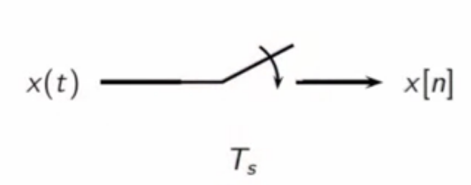
fig: raw sampling block diagram

continuous-time exponential

\[ x(t) = e^{j\Omega_0 t} ]

• always periodic; period is ( T = \frac{2\pi}{\Omega_0} )
• all angular speeds are allowed
  • unlike the discrete-time complex exponential which is limited to ([-\pi,\pi] )
• ( FT{ e^{j\Omega_0 t} } = 2 \pi \delta(\Omega - \Omega_0) )
• bandlimited to ( \Omega_0 )

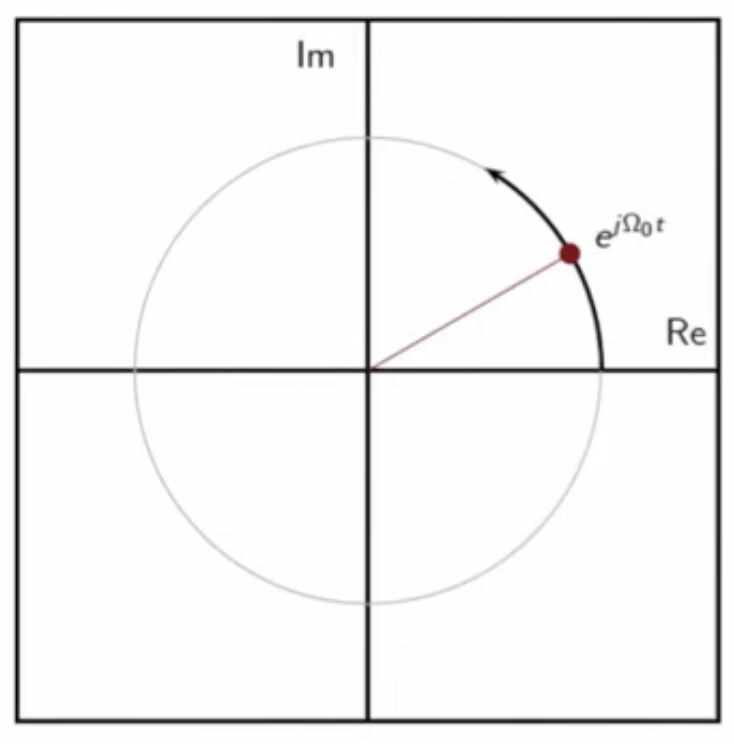
fig: continuous-time complex exponential phasor diagram on a unit circle

raw sampling with complex exponential

• raw samples are snapshots at regular intervals of the rotating point in the phasor \[ x[n] = e^{j \Omega_0 T_s n} ]
• resulting digital frequency is ( \omega_0 = \Omega_0 T_s)

phasor motion with sampling - small steps

• when (T_s < \frac{\pi}{\Omega_0} )
  • ( \omega_0 < \pi )

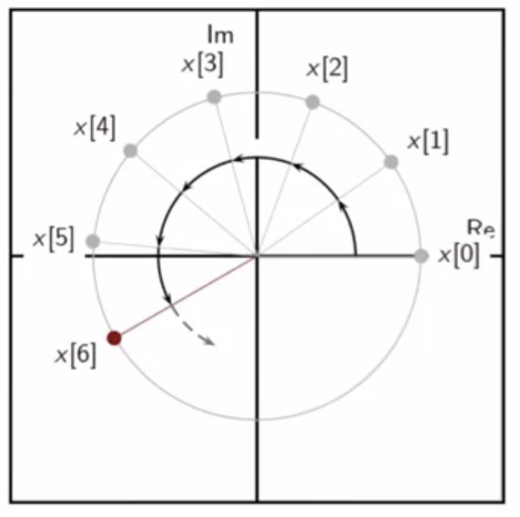
fig: sampling of continuous-time complex exponential phasor - small steps

• phasor advances forward in small steps
• appears as forward motion also
• no aliasing

phasor motion with sampling - large steps

• when ( \frac{\pi}{\Omega_0} < T_s < \frac{2\pi}{\Omega_0} )
  • ( \pi < \omega_0 < 2\pi )

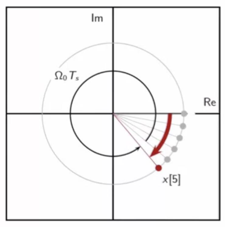
fig: sampling of continuous-time complex exponential phasor - large steps

• phasor advances forward in small steps
• appears as small steps in the backward direction
  • this is aliasing

phasor motion with sampling - very large steps

• when ( T_s > \frac{2\pi}{\Omega_0} )
  • (\omega_0 > 2\pi )

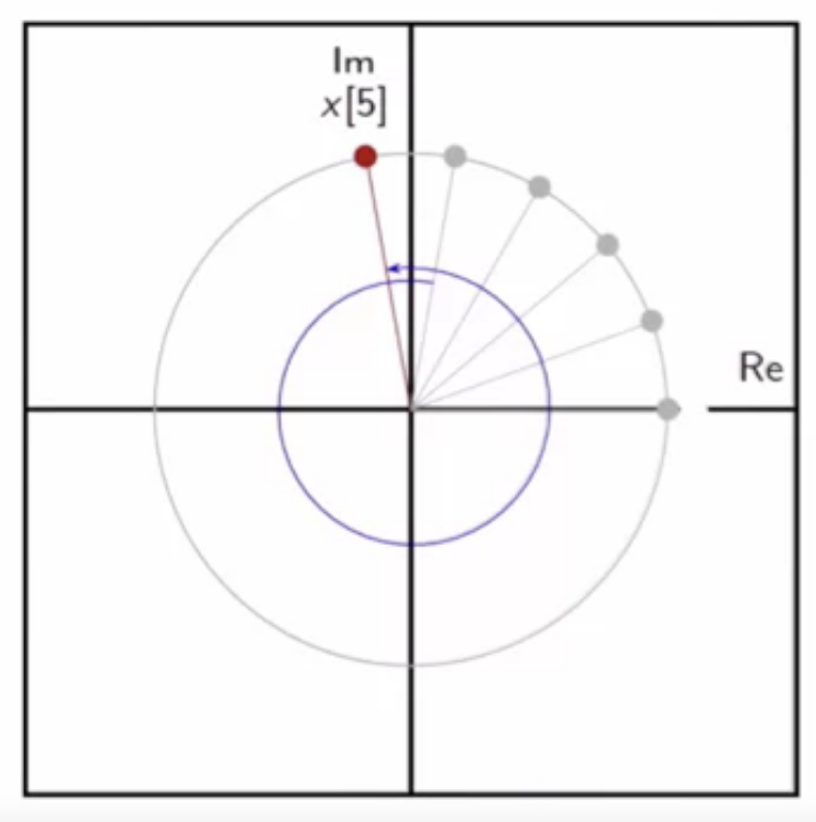
fig: sampling of continuous-time complex exponential phasor - very large steps

• phasor advances forward in larger than a full circle steps
• appears as small steps in the forward direction
• this is aliasing as well

aliasing analysis

• refer to “wagon wheel” effect
• consider the continuous-time signal ( x(t) = e^{j\Omega_0 t} )
• it is passed through a sampler sampling at equals intervals (T_s)
• then is interpolated at the same interval
• ideally, the output of this setup ( \hat{x}(t) ) should be the same as the input ( x(t) )

fig: sampling of continuous-time complex exponential phasor - very large steps

case 1

• sampling period: ( T_s , \frac{\pi}{\Omega_0} )
  • small range
• digital frequency: ( 0 < \omega_0 < \pi )
• ( \hat{x}(t) = e^{j\Omega_0 t} )
• the sampling theorem constrains are met here
• the original signal is obtained in this case

case 2

• sampling period: ( \frac{\pi}{\Omega_0} < T_s < \frac{2\pi}{\Omega_0} )
  • intermediate range
• digital frequency: ( \pi < \omega_0 < 2\pi )
• ( \hat{x}(t) = e^{j\Omega_1 t} )
  • ( \Omega_1 = \Omega_0 - \frac{2\pi}{T_s} )
• the output frequency is different from the input
  • aliasing occurs
  • conditions of the sampling theorem are not met

case 3

• sampling period: ( T_s > \frac{2\pi}{\Omega_0} )
  • large range
• digital frequency: ( \omega_0 > 2\pi )
• ( \hat{x}(t) = e^{j\Omega_2 t} )
  • ( \Omega_2 = \Omega_0 \mod (\frac{2\pi}{T_s}) )
• digital frequency shows folding back into circle angle range
• the output frequency is different from the input
  • aliasing occurs
  • conditions of the sampling theorem are not met

notes

• in aliasing, higher frequencies are windowed back into lower frequencies ranges
• sampling theorem specifies how to sample to avoid aliasing

---

sinusoidal aliasing

• consider a sinusoid [ \begin{align} x(t) & = \cos(2\pi F_0)
  F_0 &: \text{ sinusoid frequency in Hz}
  \end{align} ]
• the samples of this sinusoid is \[ \begin{align} x[n] & = x(nT_s)
  & = cos(\omega_0 n)
  \text{ sampling} & \text{ is done at multiples of } T_s
  
  F_s & = \frac{1}{T_s}
  \omega_0 & = 2\pi \bigg( \frac{F_0}{F_s} \bigg)
  \end{align} ]

sampling a sinusoid

case 1

• sampling frequency: ( F_s > 2F_0 )
  • sampling rate is more than twice the frequency of the input sinusoid
  • satisfies sampling theorem constrains
• digital frequency: ( 0 < \omega_0 > \pi )
• result: output same as input

case 2

• sampling frequency: ( F_s = 2F_0 )
  • sampling rate is at limit of sampling theorem
• digital frequency: ( \omega_0 = \pi )
• result: max digital frequency
  • ( x[n] = (-1)^n )

case 3

• sampling frequency: ( F_0 < F_s < 2F_0 )
  • sampling rate less than sampling theorem constrain
• digital frequency: ( \pi < \omega_0 < 2\pi )
• result: negative frequency
  • ( \omega_0 - 2\pi )
  • some aliasing occurs

case 4

• sampling frequency: ( F_s < F_0 )
  • sampling rate less than sampling theorem constrain
• digital frequency: ( \omega_0 > \pi )
• result: full aliasing occurs
  • ( \omega_0 \mod 2\pi )

aliasing in sinusoid sampling

• consider following sinusoid signal in continuous time domain

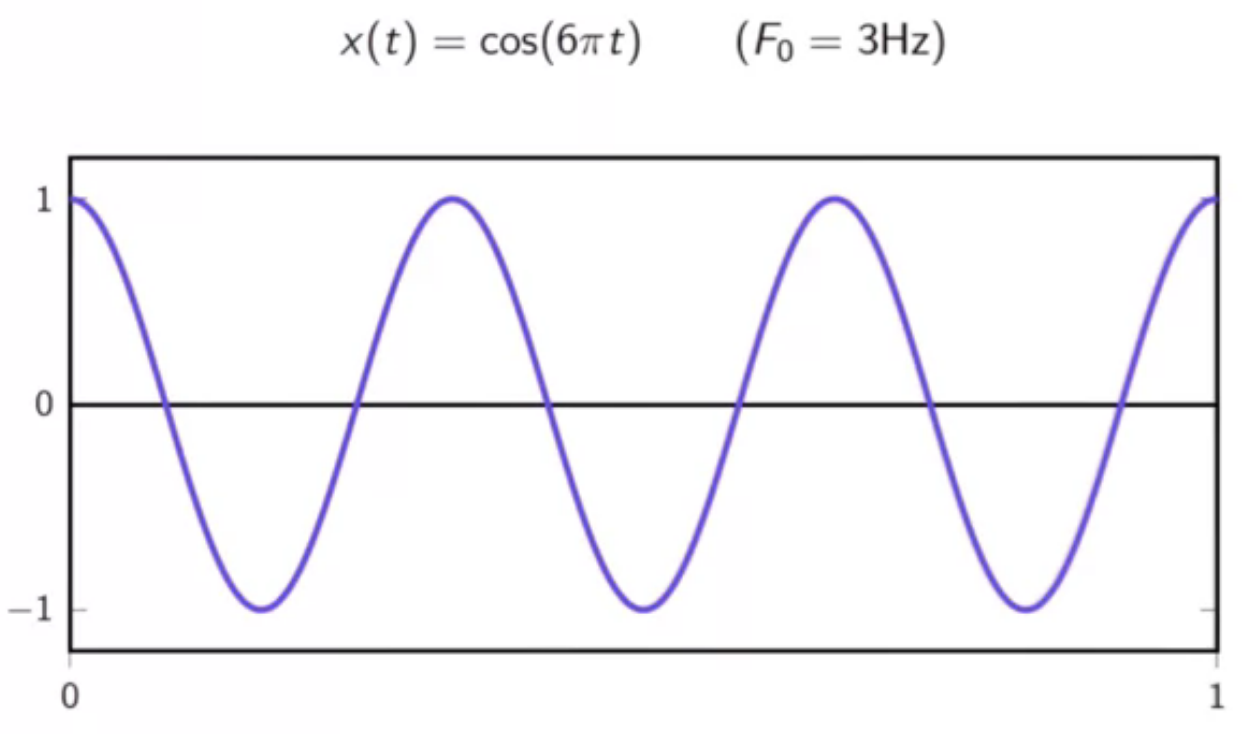
fig: sinusoid signal to be sampled

• as per sampling theorem,
  • this signal may be perfectly reconstructed with sampled data only if
  • sampling frequency is atleast (2F_0)
  • i.e. ( F_s \geq 6 Hz)

(F_s = 100 Hz)

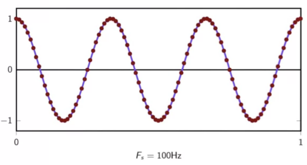
fig: very large sampling frequency

(F_s = 50 Hz)

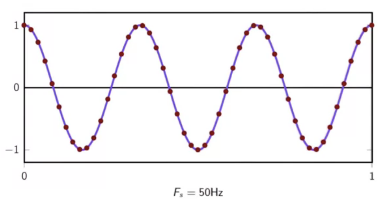
fig: fairly large sampling frequency

(F_s = 10 Hz)

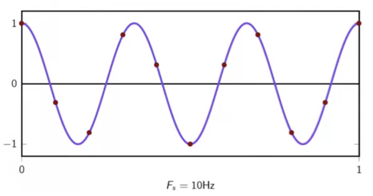
fig: comfortably sufficient sampling frequency

(F_s = 6 Hz)

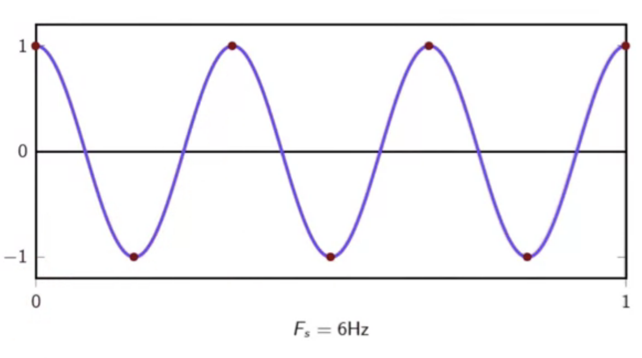
fig: limit sampling frequency

(F_s = 2.9 Hz)

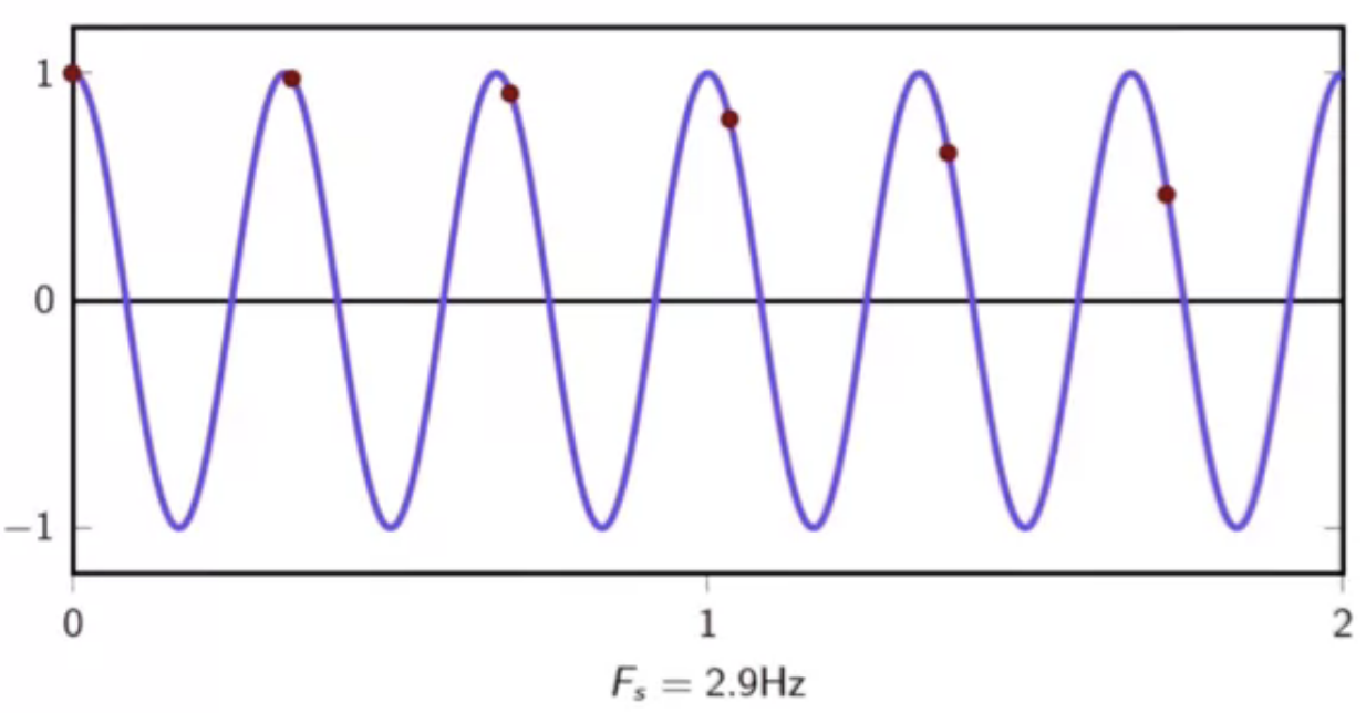
fig: lower than limit sampling frequency

observations

• at higher than limt frequencies of sampling, the input sinusoid signal is adequately represented
  • this enables accurate reconstruction from samples
• at limit, it is maximum digital frequency
• while theoretically it is above the limit, it doesn’t carry sufficient information for a perfect resonstruction
• some other information about the quality of the signal has to be known
  • i.e. that a sinusoid was sampled
  • if this is not known a triangular curve may be fit in for example
• at frequencies below the sampling theorem limit, the input signal is poorly represented
• stretching the interval longer we see that the samples actually gain a new frequency
  • at sampling frequency 2.9 Hz for a signal of 3 Hz
    • the samples gain a frequency of 0.1 Hz
    • in the opposite direction
  • this is the modulo of the two frequencies 2.9 Hz mod 3 Hz = -0.1
• the plots below are static snapshots
  • in a moving sinusoid plot, the frequency of the reconstructed wave would be backwards

fig: below limit sampling frequency - interval of 2

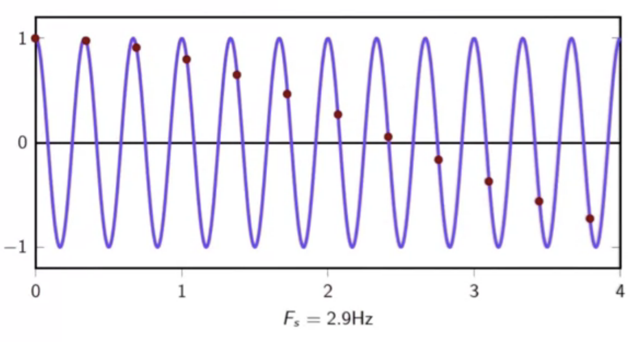
fig: below limit sampling frequency - interval of 4

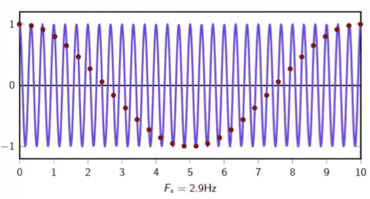
fig: below limit sampling frequency - interval of 10

---

aliasing for arbitrary spectra

• aliasing samples introduce superfluous information during interpolation
• they do not accurately represent the original
• this is not ideal in practice, so aliasing is to be avoided
• consider raw sampling of an arbitrary signal
  • here the samples are ( x[n] = x_c(nT_s) )

fig: raw sampling block diagram

• in the fourier transform spectrum

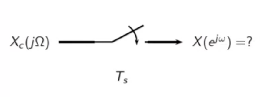
fig: raw sampling block diagram - frequency domain

• need a general expression for the spectra of arbitrary signals sampled to sequences
  • that relates the input signal spectrum (input CTFT)

setup sampling system

• pick sampling interval (T_s)
• set ( \Omega_N = \frac{\pi}{T_s} )
• pick ( \Omega_0 < \Omega_N )
  • ( \Omega_0 ): Signal Frequency
  • ( \Omega_N ): Nyquist Frequency

sampling system operation analysis

• consider input to sampling system
  • regenerated signal is faithfully reproduced

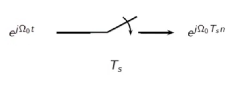
fig: raw sampling block diagram - frequency domain

• consider input with a different, higher that nyquist frequency

fig: raw sampling block diagram - frequency domain

• the output may be reduced

fig: raw sampling block diagram - frequency domain

• this looks like lower frequency output
• it has fallen back to the module window of the circle

fig: raw sampling block diagram - frequency domain

general case

• the aliasing frequency can be generalized as follows

fig: raw sampling block diagram - frequency domain

spectrum of raw sampled signals

• take fourier transform of the sampled sequence

\[ \begin{align} x[n] & = x_c(nT_s) _
& = \frac{1}{2\pi} \int{-\infty}{\infty} X_c(j\Omega) e^{j\Omega n T_s} d\Omega
\end{align} ]

• frequencies that are (2\Omega_N) apart are aliased
  • the integration interval is split to reflect this

\[ \begin{align} x[n] & = \frac{1}{2\pi} \sum_{k = -\infty}^{\infty} \int_{(2k-1)\Omega_N}^{(2k+1)\Omega_N} X_c(j\Omega) e^{j\Omega n T_s} d\Omega
\end{align} ]

• anything at and beyond (2\Omega_N ) is folded back

fig: frequency folding

fig: frequency folding in ( 2\Omega_N )

fig: frequency folding in ( 4\Omega_N )

• with a change of variable and using ( e^{j(\Omega + 2 k \Omega_N) T_s n} = e^{j \Omega T_s n} ) \[ \begin{align} x[n] & = \frac{1}{2\pi} \sum_{k = -\infty}^{\infty} \int_{-\Omega_N}^{\Omega_N} X_c(j (\Omega - 2k\Omega_N)) e^{j\Omega n T_s} d\Omega _
  & = \frac{1}{2\pi} \int{-\Omega_N}^{\Omega_N} \bigg[ \sum_{k = -\infty}^{\infty} X_c(j (\Omega - 2k\Omega_N)) \bigg] e^{j\Omega n T_s} d\Omega
  \end{align} ]
• to periodize this spectrum

[ \begin{align} \tilde{X_c} (j \Omega) & = \sum_{k = -\infty}^{\infty} X_c(j (\Omega - 2k\Omega_N)) _
\text{ such that } & _
_x[n] & = \frac{1}{2\pi} \int{-\Omega_N}^{\Omega_N} \tilde{X_c}(j\Omega) e^{j\Omega n T_s} d\Omega
\end{align} ]

• change of variable ( \omega = \Omega T_s )

\[ \begin{align} x[n] & = \frac{1}{2\pi} \int_{-\pi}^{\pi} \tilde{X_c} \bigg( j \frac{\omega}{T_s} \bigg) e^{j\omega n} d\omega _
& = IDTFT \bigg{ \frac{1}{T_s} \tilde{X_c} \bigg( j \frac{\omega}{T_s} \bigg) \bigg} _
_2\pi\text{-periodic; } & \text{so, a valid DTFT} _
_X(e^{j\omega}) & = \frac{1}{T_s} \sum{k = -\infty}^{\infty} X_c \bigg( j \frac{\omega}{T_s} - j \frac{2\pi k}{T_s} \bigg) \end{align} ]

• thus obtained is the DTFT of the sampled sequence
  • in relation to the CTFT of the input signal

bandlimited example

bandlimited to ( \Omega_0 ) and ( \Omega_N > \Omega_0 )

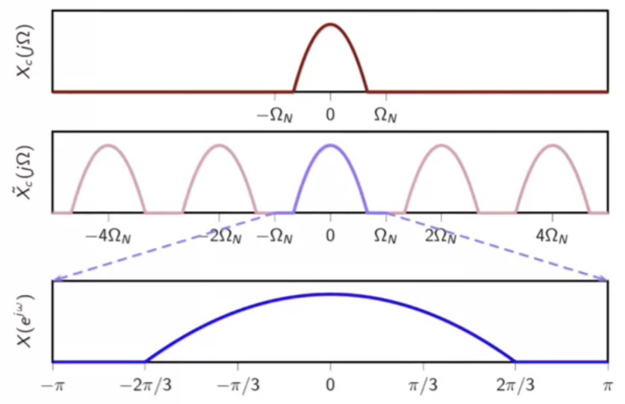
fig: CTFT, periodic CTFT, and sampled DTFT - meets sampling theorem criteria

bandlimited to ( \Omega_0 ) and ( \Omega_N = \Omega_0 )

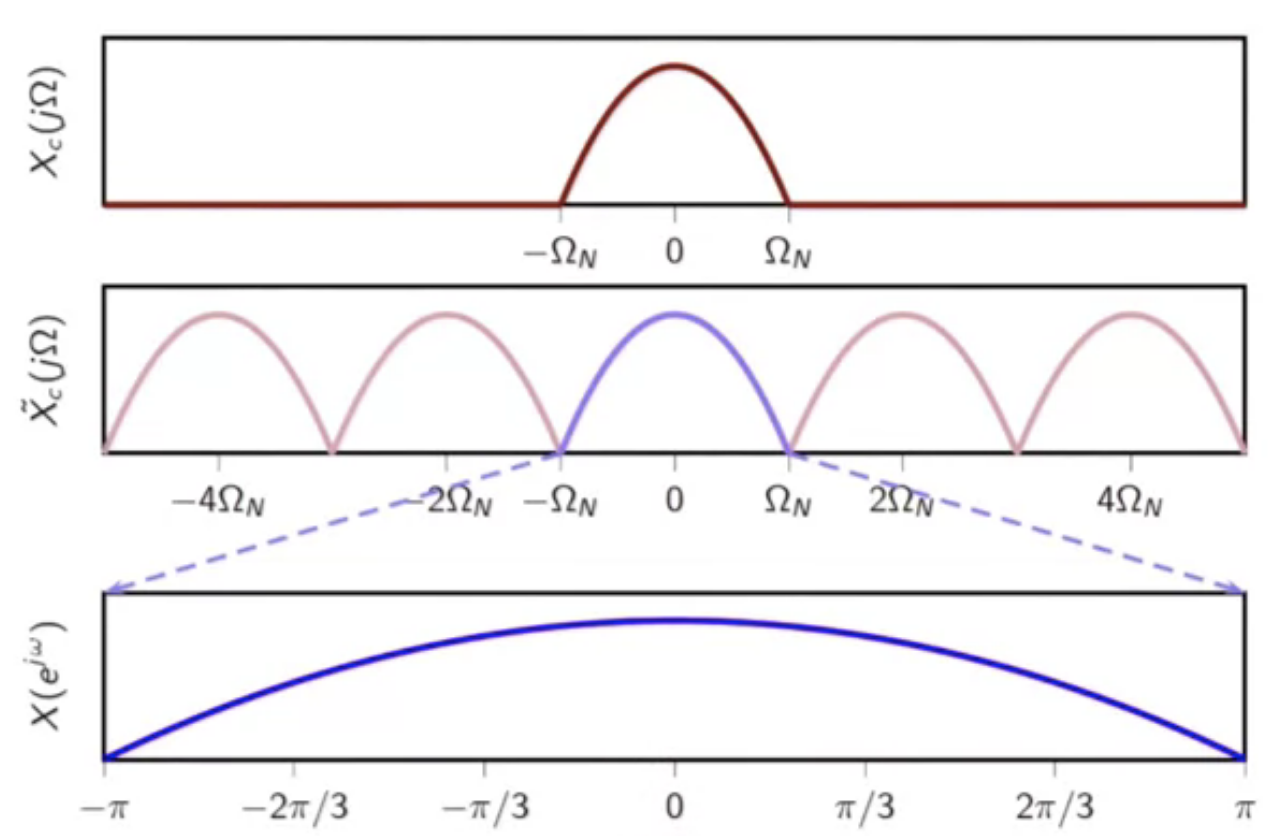
fig: CTFT, periodic CTFT, and sampled DTFT - at limit

bandlimited to ( \Omega_0 ) and ( \Omega_N < \Omega_0 )

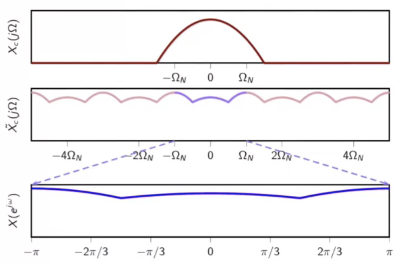
fig: CTFT, periodic CTFT, and sampled DTFT - flouts sampling theorem criteria

non-bandlimited example

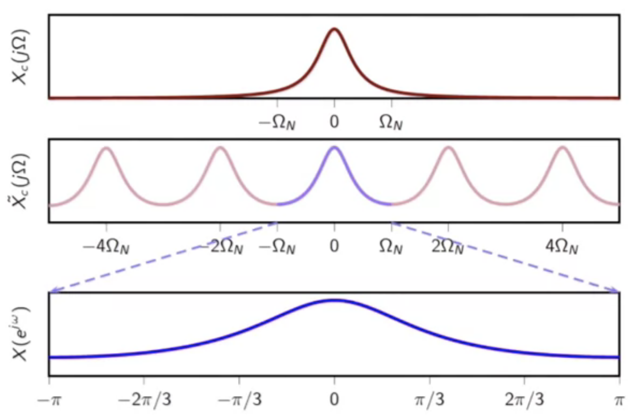
fig: CTFT, periodic CTFT, and sampled DTFT

---

sampling strategies

• for a given sampling interval (T_s)
  • the sampling strategy a depends on if the given signal is bandlimted or not
• if bandlimited to (\frac{\pi}{T_s} ) or less, choose raw sampling
  • this equivalent to sinc sampling up to a scaling factor (T_s)
• if signal is not bandlimited, one of two paths may be chosen
  • bandlimit by passing signal through lowpass filter in continuous-time domain
    • then sample with sinc sampling
  • else raw sample and incur aliasing
    • alias is not so great, so the other option is generally chosen

sinc sampling and interpolation

• in sinc sampling, the inner product between a properly scaled and shifted sinc function with the signal provides sample value
• this is equivalent to first passing the signal through an ideal lowpass filter with cutoff frequency ( \Omega_N = \frac{\pi}{T_s} )
  • then taking a sample every (T_s) seconds

[ \begin{align} & \text{ sampled signal: }
\hat{x_n} & = \langle sinc \bigg( \frac{t - nT_s}{T_s}, x(t) \bigg) \rangle _
& = (sinc{T_s} * x)(n T_s) _
_
_& \text{ interpolation of sampled signal: } _
_\hat{x}(t) & = \sum{n} x[n] sinc \bigg( \frac{t - nT_s}{T_s} \bigg)
\end{align} ]

fig: lowpass bandwidthing - sampling - sinc interpolation

least-squares approximation

• looking at the sampling and interpolation scheme purely geometrically
• consider continuous signal and the BL space with orthonormal sinc basis

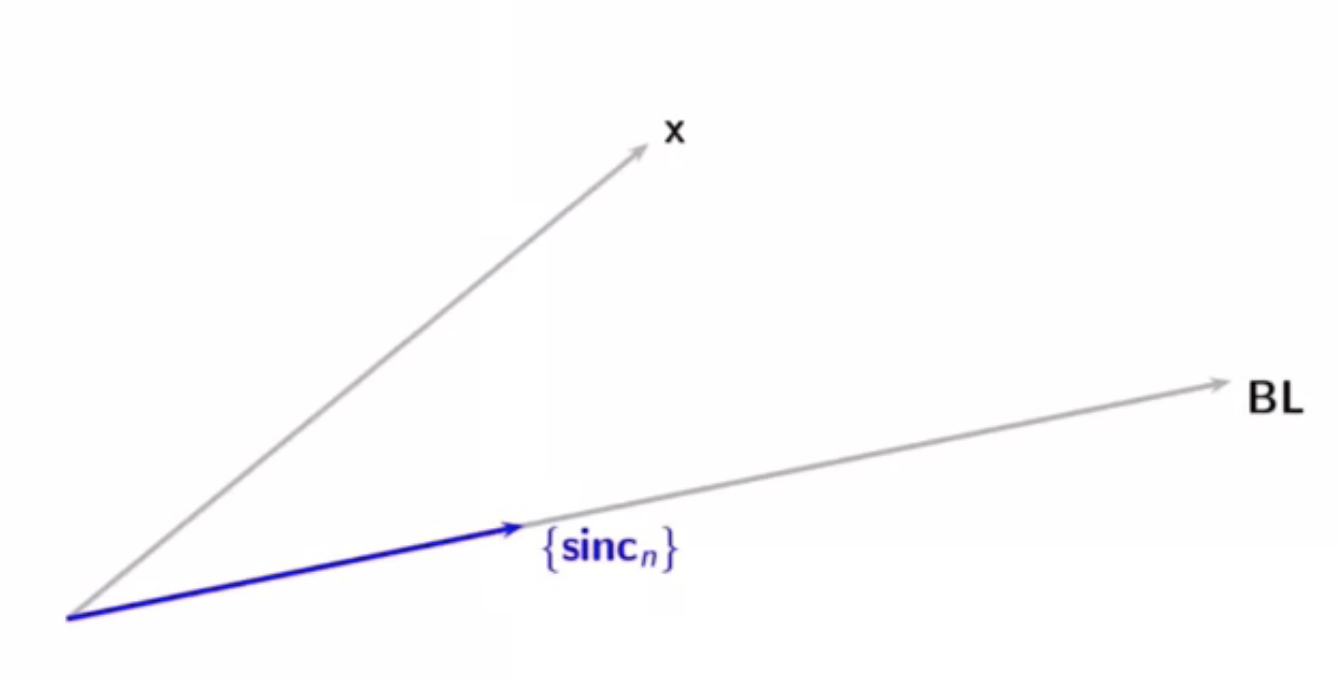
fig: BL space and continuous-time input signal

• consider an orthonormal project of the continuous time input signal on to the BL space
• the expansion is seen below

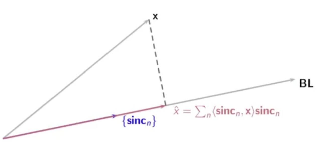
fig: projection of continuous-time input signal on to BL space

example

• consider frequency spectrum of continuous-time signal

fig: spectrum of continuous-time input signal

• this is then lowpass filtered

fig: lowpass filter on the continuous-time input signal

• to obtain a bandlimited spectrum

fig: bandlimited continuous-time input signal

• then the bandlimitied spectrum is smapled
• this leads to a periodic spectrum

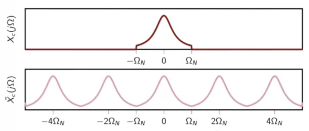
fig: sampled signal periodic spectrum

• the DTFT of this sampled sequence is examined
• this is (2\pi) periodic

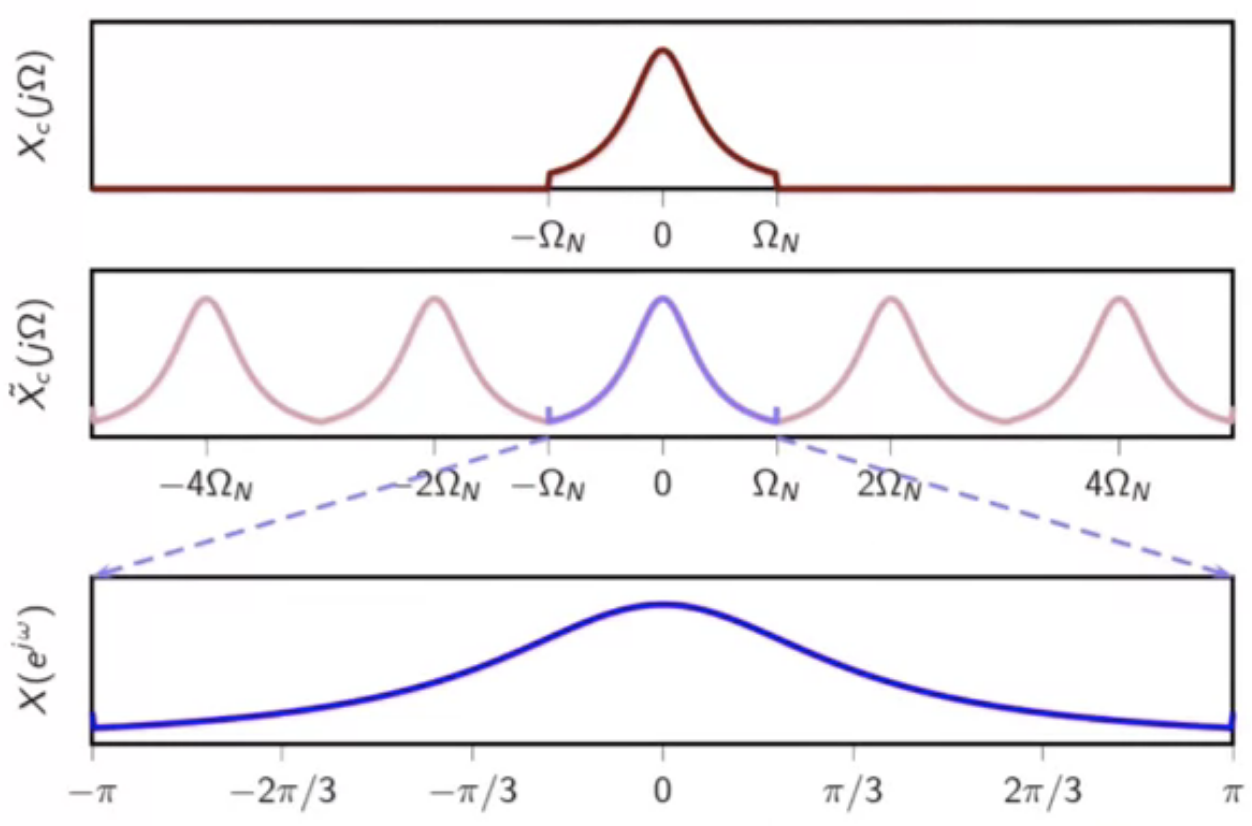
fig: DTFT of the sampled sequence

• this is then re-interpolated into continuous-time using sinc interpolation
  • this is the exact match of the bandlimited version of the input signal
  • this is the orthogonal projection of the original signal in the space of BL signals

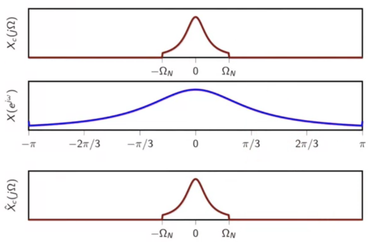
fig: DTFT of the sampled sequence

---

references

• ecole dsp - filters