[DSP] W07 - Quantization
contents
- the first half of dsp is the discretisation of time, i.e., sampling.
- the second half is quantization
- digital devices can only deal with integers no matter how many bits are used
- so, the numeric range of the finite samples has to mapped on to a set of finite values
- in doing so, there is an irreversible loss of information
- the quantizer introduces noise
stochastic signal processing
- stochastic: random
- random signals need processing in the real-world
- deterministic signals are known in advance
- many interesting signals are known in advance
- only a few things about it are known
- eg: speech signal
- stochastic signals are described probabilistically
- such random signals can be dsped as well
single discrete-time random signal generator
- a fair coin toss \[ x[n] = \Bigg{ \begin{matrix} +1 & \text{ n-th toss is head } \ -1 & \text{ n-th toss is tail } \end{matrix} ]
- each sample is independent of the other
- each sample has 50% probability
- each time the generator is run, the signal is realized differently
- the mechanism behind each instance is know
- but that particular realization is not known before hand
- this can be analyzed spectrally
DFT of a random signal
- explore DFT of finite set of samples of a random signal
- every time the experiment is repeated, the result is different
- longer realizations may be experimented with
averaging
- when faced with random data, an intuitive approach is to take “averages”
- in probability theory the average is across different realizations of the experiment, not across the time axis
- this is called the expectation (E[x[n]])
- for the coin-toss signal
\[ \begin{align}
E[x[n]] & = -1 P[\text{n-th toss is tail}] + 1 P[\text{n-th toss is head}]
& = 0
\end{align} ] - so the average value for each sample is zero
- so averaging the DFT values will not work as (E[x[n]] = 0)
- however, the signal does move, so it;s energy or power must be non-zero
random energy and power
- the coin toss signal has infinite energy
[ \begin{align}
E_x & = \lim_{N \rightarrow \infty } \sum_{n = -N}^{N} \vert x[n] \vert^2 _
& = \lim{N \rightarrow \infty } (2N + 1)
& = \infty
\end{align} ] - power is finite over an interval
[ \begin{align}
P_x & = \lim_{N \rightarrow \infty } \frac{1}{2N + 1} \sum_{n = -N}^{N} \vert x[n] \vert^2
& = 1
\end{align} ]
power spectral density
- try to average DFT square magnitude, normalized
- pick an interval length (N)
- pick a number of iterations (M)
- tun the signal generator (M) times
- to obtain ( M ) (N)-point realizations
- compute the DFT of each realization
- average their square magnitude divided by (N)
- this yields the following results
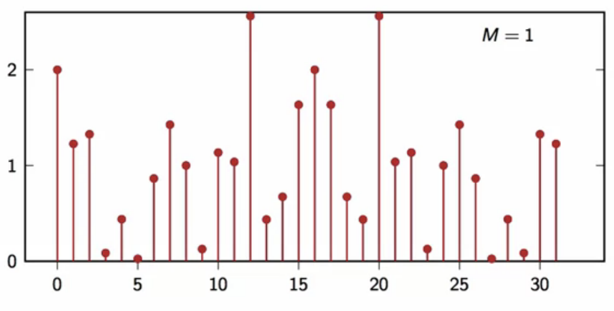
fig: DFT average plot (M = 1)
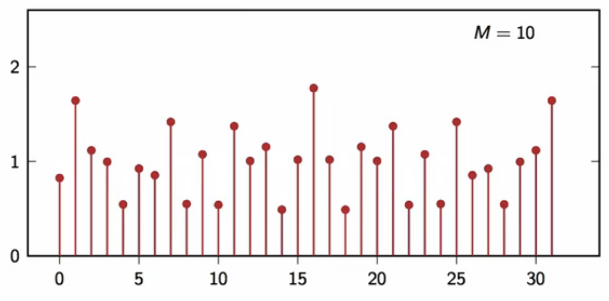
fig: DFT average plot (M = 10)
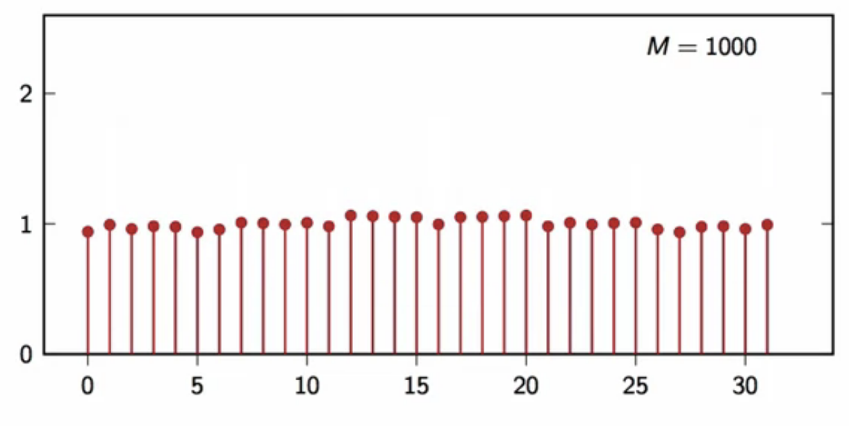
fig: DFT average plot (M = 1000)
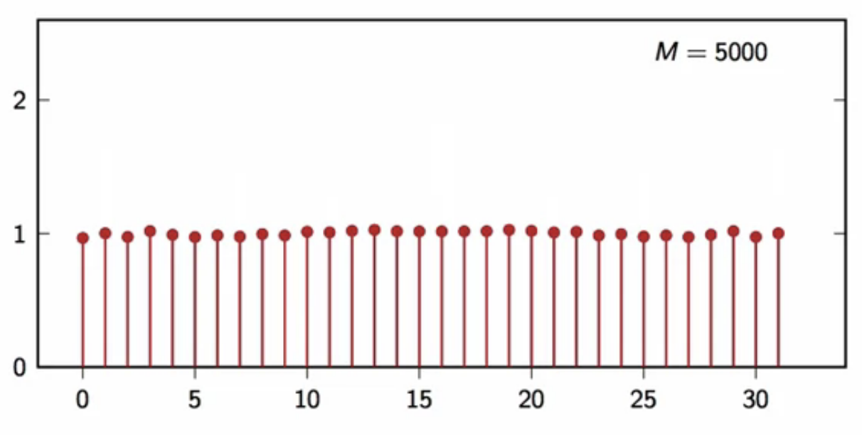
fig: DFT average plot (M = 5000)
- this is the definition of the power spectral density \[ P[k] = E[\frac{\vert X_N[k]\vert^2}{N}] ]
- this looks very much like (P[k] = 1)
- if (\vert X_N[k]\vert^2) tends to the energy distribution in frequency
- (\frac{\vert X_N[k]\vert^2}{N}) tends to the power distribution
- i.e. density in frequency
- the frequency-domain representation for stochastic process is the power spectral density
intuition
- (P[k]=1) means that power is equally distributed over all frequencies
- i.e. we cannot predict if the signal moves ‘slow’ or ‘suprfast’
- this is because each sample is independent of the others
- a given realization could
- be all ones
- or the sign changes alternate sample
- or anything in between
- this is also the description of “luck”
filtering a random signal
- consider a 2-pt moving average filter \[ y[n] = \frac{(x[n] + x[n-1]}{2} ]
- a random signal (x[n] ) is filtered with this
- following is the power spectral density of the output of this filter
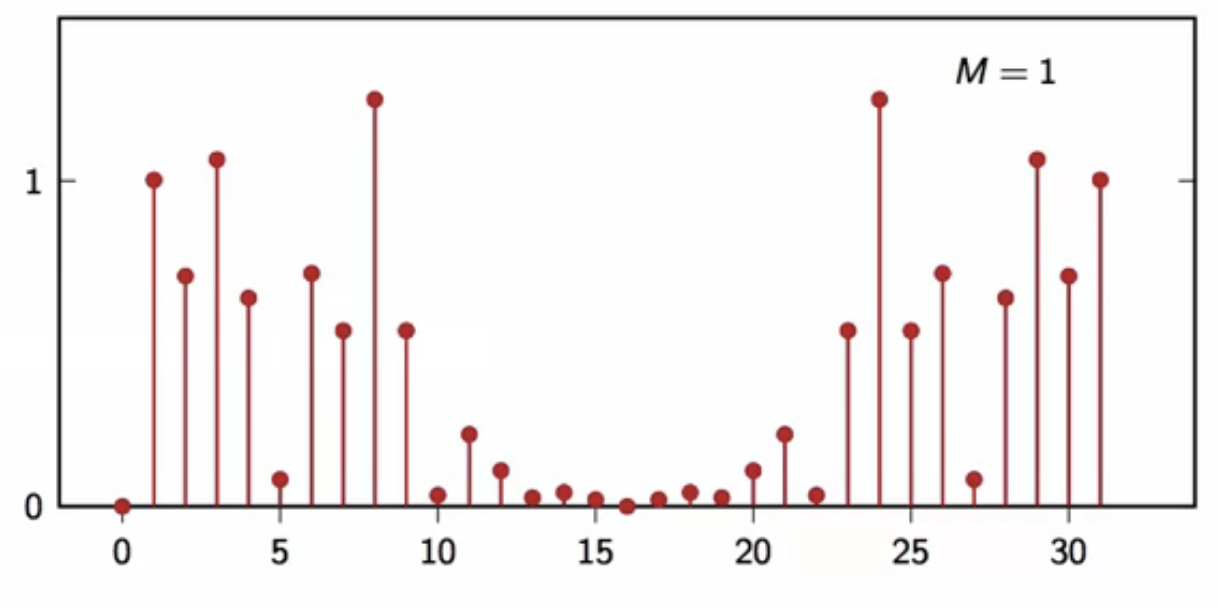
fig: moving average filtered output DFT average (M = 1)
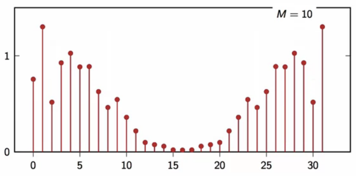
fig: moving average filtered output DFT average (M = 10)
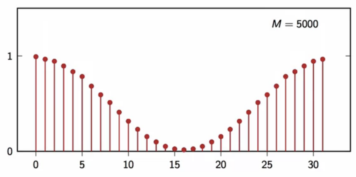
fig: moving average filtered output DFT average (M = 5000)
- as the number of realizations used to compute the average increases, the shape converges
- the shape it converges to is defined below
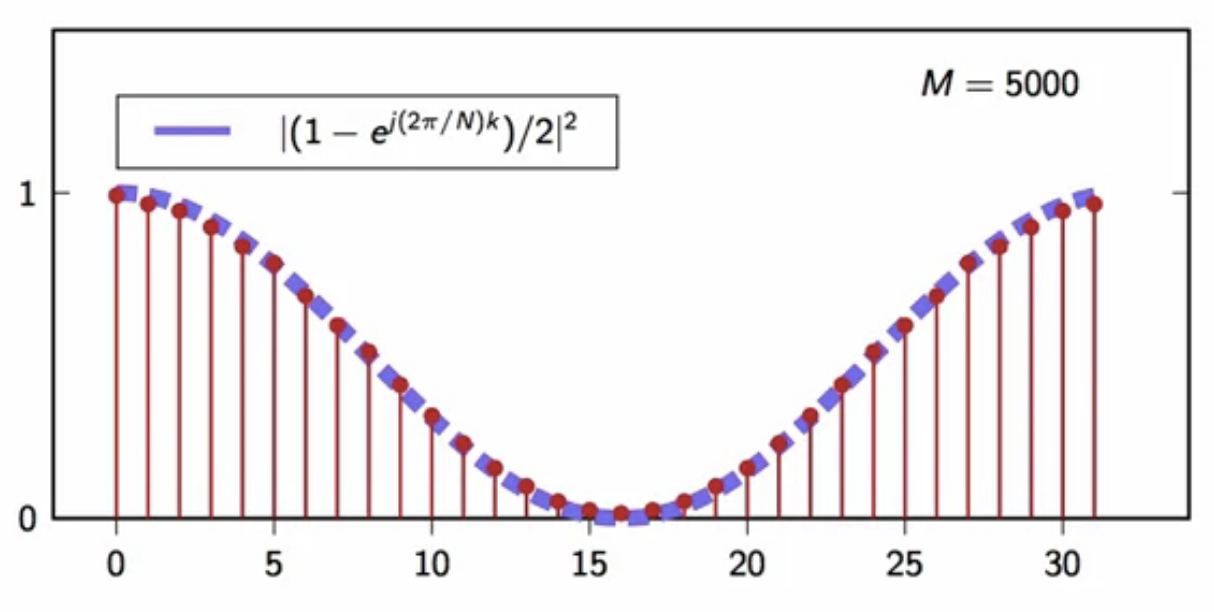
fig: moving average filtered output DFT average (M = 5000) - convergence shape
- the power spectral density of the output is the product of the power spectral density of the input scaled by the squared magnitude of the filter frequency response \[ P_y[k] = P_x[k] \vert H[k] \vert^2 \text{, where } DFT{h[n] } ]
- this result may be generalized beyond a finite set of samples
- the world of infinite support stochastic processes
generalization
- a stochastic process is characterized by its power spectral density (PSD)
- it may be shown that PSD:
\[ P_x(e^{j\omega}) = DTFT{ r_x[n] }
]
- where:
- ( r_x[n] = E[x[k]x[n+k]] ) is the autocorrelation of the process
- where:
- for a filtered stochastic process ( y[n] = \mathcal{H} { x[n] } ), it is \[ P_y(e^{j\omega}) = \vert H(e^{j\omega}) \vert^2 P_x(e^{j\omega}) ]
- this means that the filters designed for deterministic case still work in stochastic case
- only in magnitude
- the concept of phase is lost however, since the shape of a realization is not known in advance
- only the power distribution across frequencies is known
noise
- it’s everywhere
- thermal noise
- sum of extraneous interferences
- quantization and numerical errors
- we can model noise as a stochastic signal
- since the noise source is not known
- the most important noise is white noise
white noise
- “white” indicates uncorrelated samples
- so autocorrlation of noise signal is zero everywhere except zero - where it is the variance of the signal \[ r_w[n] = \sigma^2\delta[n] ]
- has zero mean
- the power spectral density is a constant
- is equal to the variance of the process \[ P_w(e^{j\omega}) = \sigma^2 ]
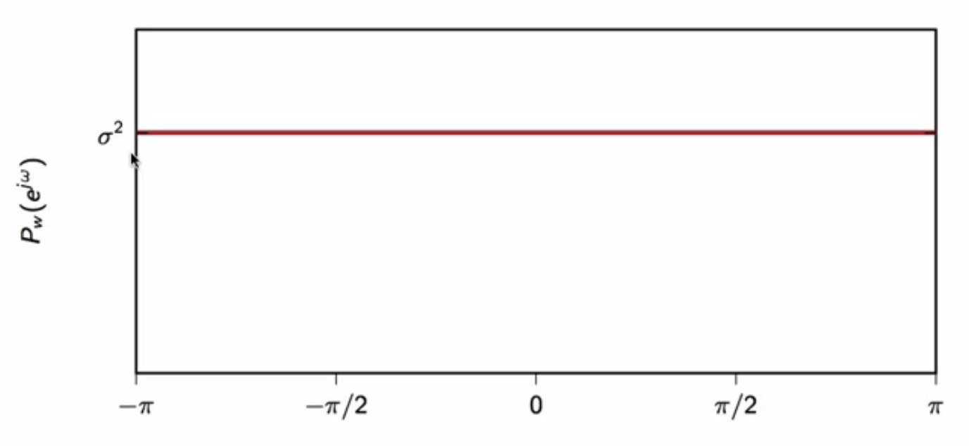
fig: power spectral density of white noise
- the power spectral density of white noise is independent of the probability distribution of the signal samples
- depends only on the variance
- distribution is important to estimate bounds of the signal
- in the time domain
- very often, a gaussian distribution models the experimental data the best
- represents many unknown additive sources of noise well
- AWGN: additive white gaussian noise
quantization
- this the second half of the story of dsp
- digital devices can only deal with integers
- (b) bits per sample
- the range of a signal is to be mapped onto a finite set of values
- this causes an irreversible loss of information
- termed quantization noise
- the finite set of values is the resolution of the system
quantizer
- a quantizer takes in a discrete-time samples (x[n] \in \mathbb{C} )
- it outputs integers ( \hat{x}[n] \in \mathbb{N} )
- the output is said to be quantized version of the input discrete-time sequence

fig: a quantizer block diagram representation
- quantization considerations
- storage budget
- how many bits to allocate be sample
- storage scheme
- fixed point vs floating point
- properties of input
- range
- probability distribution
- storage budget
scalar quantizer
- it is the simplest quantizer
- each sample is encoded individually
- hence termed scalar
- each sample is encoded independently
- memoryless quantization
- each sample is encoded using (R) bits
- each sample is encoded individually
scaler quantizer operation
- assume input signal bounded: ( A \leq x[n] \leq B ) for all (n)
- each sample quantized over ( 2^R ) possible values
- (R) bits per sample being used
- in ( 2^R ) intervals
- each interval associated to a quantization value
 fig: quantization into fixed intervals
- each sample quantized over ( 2^R ) possible values
example: (R = 2)
- range (A-B) is divided into 4 intervals
- ( i_k ) mark the boundaries of each interval
- ( \hat{x}_k ) is the representative value of each interval
- each interval is encoded into two bits
- first interval: ( k = 00 )
- second interval: ( k = 01 )
- third interval: ( k = 10 )
- fourth interval: ( k = 11 )
- so the real value that represents an interval is associated with corresponding bit by the quantizer internally

fig: quantization into fixed intervals
- optimization considerations;
- interval boundaries ( i_k )
- quantization values ( \hat{x}_k )
quantization error
- quantization error is the difference between the representative value and the real value
\[ \begin{align}
e[n] & = \mathcal{Q}{ x[n] } - x[n]
& = \hat{x}[n] - x[n]
\end{align} ] - assumptions for preliminary analysis of error:
- the input ( x[n] ) is modelled as a stochastic process
- the error is modelled as white noise
- error samples are uncorrelated
- all error samples have the same distribution
- assumptions are pretty drastic, but provide worst-case scenario insight
- input statistical description is needed
- assumptions for the internal structure of the quntizer:
- uniform quantizaton
- range is spilt into equal intervals
- number of intervals: ( 2^R )
- width of interval: ( \Delta = (B-A)2^{-R} )

fig: ( R=2 ) quantization intervals in range
- mean-square-quantization-error is given by variance
[ \begin{align}
\sigma_e^2 & = E[\vert \mathcal{Q} { x[n] } - x[n] \vert^2 ] _
& = \int{A}^{B} f_x(\tau)(\mathcal{Q} { \tau } - \tau )^2 d\tau _
& = \sum{k=0}^{2^R - 1} \int_{I_k} f_x(\tau) (\hat{x}_k - \tau)^2 d\tau
\end{align} ] - error depends on the probability distribution of the input
- this needs to be known to evaluate quantization mse
- continuing with more assumptions for this analysis…
- the input is assumed to be uniformly distributed
- input’s probability distribution function is a constant over the range (A-B)
- with amplitude ( \frac{1}{B-A} )
- input’s probability distribution function is a constant over the range (A-B)
- with this assumption about the input, the mse therefore becomes
[ \begin{align}
\sigma_e^2 & = \sum_{k=0}^{2^R - 1} \int_{I_k} \frac{(\hat{x}_k - \tau)^2}{B-A} d\tau
\end{align} ] - to find the optimal quantization point, this quantization mse is minimized
[ \begin{align}
\frac{ \partial \sigma_e^2 }{ \partial \hat{x_m} } & = \frac{ \partial }{ \partial \hat{x_m}} \sum_{ k = 0}^{ 2^R - 1} \int_{I_k} \frac{(\hat{x_k} - \tau)^2}{B-A} d\tau _
& = \int{I_m} \frac{ 2( \hat{x_k} - \tau) }{ B - A } d\tau _
& = \frac{ (\hat{x_m} - \tau)^2 }{B - A} \Bigg \vert{A + m \Delta }^{ A + m\Delta + \Delta}
\end{align} ] - to minimize the error, set partial derivative of error to zero
[ \begin{align}
\frac{\partial \sigma_e^2}{\partial\hat{x_m}} = 0 & \text{ for } \hat{x_m} = A + m\Delta + \frac{\Delta}{2}
\end{align} ] - so optimal quantization point for all intervals is the interval’s midpoint
quantizer characteristic
- below is a 3 bits per sample quantizer characteristic
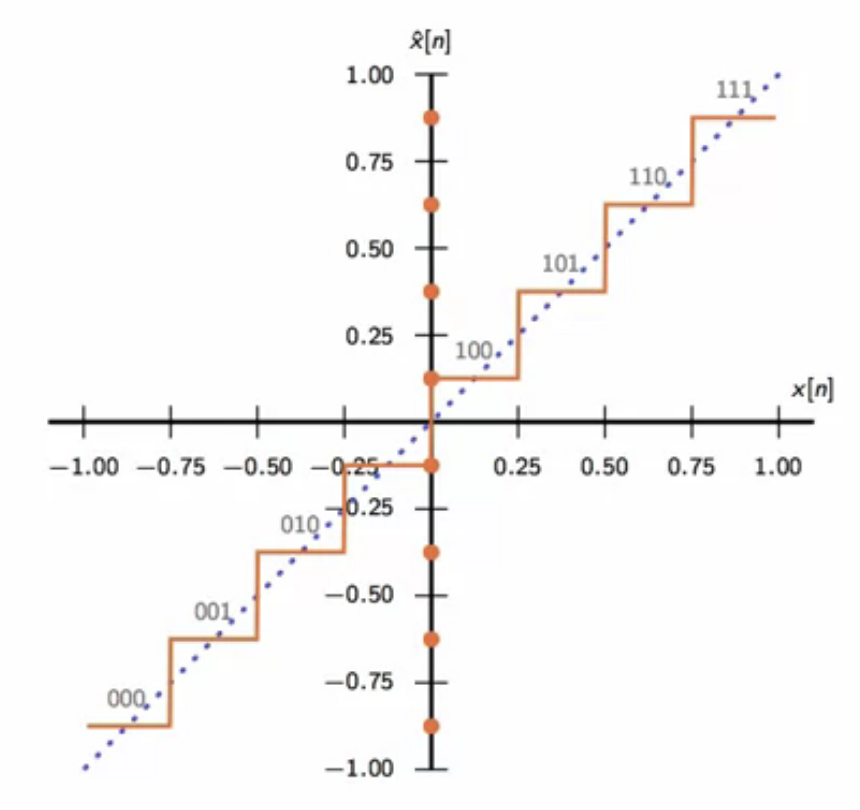
fig: uniform 3-bit (R=3) quantizer characteristic
- quantizer mse is
[ \begin{align}
\sigma_e^2 & = \sum_{k = 0}^{2^R - 1} \int_{A + k\Delta}^{A + k\Delta + \Delta} \frac{ (A + k \Delta + \frac{\Delta}{2} - \tau)^2}{B - A} d\tau
& = 2^R \int_0^\Delta \frac{(\frac{\Delta}{2} - \tau)^2}{B-A} d\tau
& = \frac{\Delta^2}{12}
\end{align} ]
error analysis
- error energy \[ \sigma_2^2 = \frac{\Delta^2}{12} ]
- signal energy \[ \sigma_x^2 = \frac{(B-A)^2}{12} ]
- signal to noise ratio \[ SNR = 2^{2R} ]
- signal to noise ratio in (dB) [ SNR_{dB} = 10 \log_{10}^{2^{2R}} \approx 6R dB ]
6dB/bit rule of thumb
- a CD has 16 bits/sample
- max SNR = 96dB
- a DVD has 24 bits/sample
- max SNR = 144dB