[DSP] W08 - Digital Communication Systems

contents

• success factors
• analog channel constraints
  • channel capacity
  • channel capacity examples
• communication system design
  • transmitter design
• bandwidth control
  • multirate techniques
  • fitting the transmitter spectrum
  • raised cosines
• power control
  • probability of error
  • pulse amplitude modulation (PAM)
  • quadrature amplitude modulation (QAM)

---

• from source to destination, a signal goes through many incarnations
• it travels through a variety of analog communication channels
  • wireless, copper wire, optical fibre, et
  • each channel has a set of constraints the signal must adheres to
• signal can undergo various transformations, such as conversion from analog to digital and later back to analog or signal regeneration

digital data throughput through time

• Transatlantic Cable
  • 1866: 8 words per minute
    • $\approx 5bps$
  • 1956: AT&T, co-ax cable with 48 voice channels
    • $\approx 3Mbps$
  • 2005: Alcatel Tera10, fiber
    • 8.4 Tbps ( $8.4X{10}^{12}$ )
  • 2012: fiber
    • 60 Tbps
• Voiceband modems
  • 1950s: Bell 202
    • 1200 bps
  • 1990s: V90
    • 56 Kbps
  • 2008; ADSL2+
    • 24 Mbps

---

success factors

distinctions of the DSP paradigm

• integers are easy to regenerate
• good phase control with digital filters
• adaptive algorithms can be seamlessly integrated into DSP systems
  • procedures that adapt behavior in response to received signal

algorithmic nature of DSP synergizes with information theory

• JPEG’s entropy coding
  • discrete cosine transform matched seamlessly to information theory techniques
  • techniques from different domains combined produces powerful algorithms
• CD and DVD error corrections
  • encoding acoustic info matched to error corrector codes
  • even scratched cds and dvds play
• trellis-coded modulation and viterbi decoding
  • analog channels are taken advantage of in communication systems with these techniques

hardware advancements

• miniaturization of signal processing hardware
  • moore’s law
• general-purpose platforms available
  • no need to make customized hardware for specific application
  • modular assembly of off-the-shelf hardware provides custom solutions
• power efficiency
  • many communications channels can be processed by relatively small data centers

---

analog channel constraints

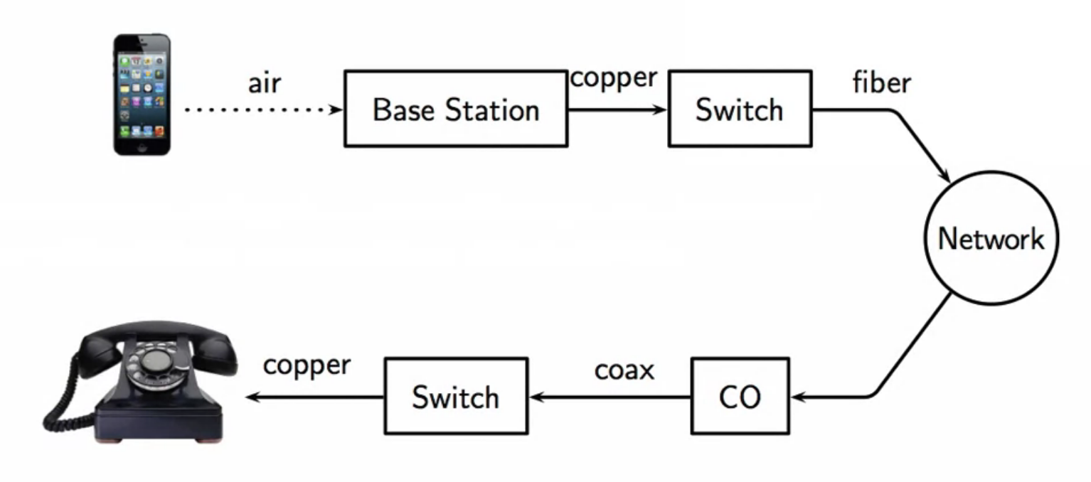
fig: signal flow in a real world communication system

• channels used:
  • air
  • copper
  • fiber
  • coax
  • copper
• the signal goes through changes to be able to travel through the channel chain

channel capacity

• unescapable limits of physical channels that affects the capacity of the channel
  • bandwidth constraints
    • signal will have to be limited to certain frequency band
  • power constraint
    • power over given bandwidth cannot be arbitrary
    • there will be limits
• channel capacity is the the maximum amount of information that can be reliably delivered over a channel
  • usually in bits per second
• the specifications of the channel is given to communication system engineers
  • to reliably transmit information over the channel

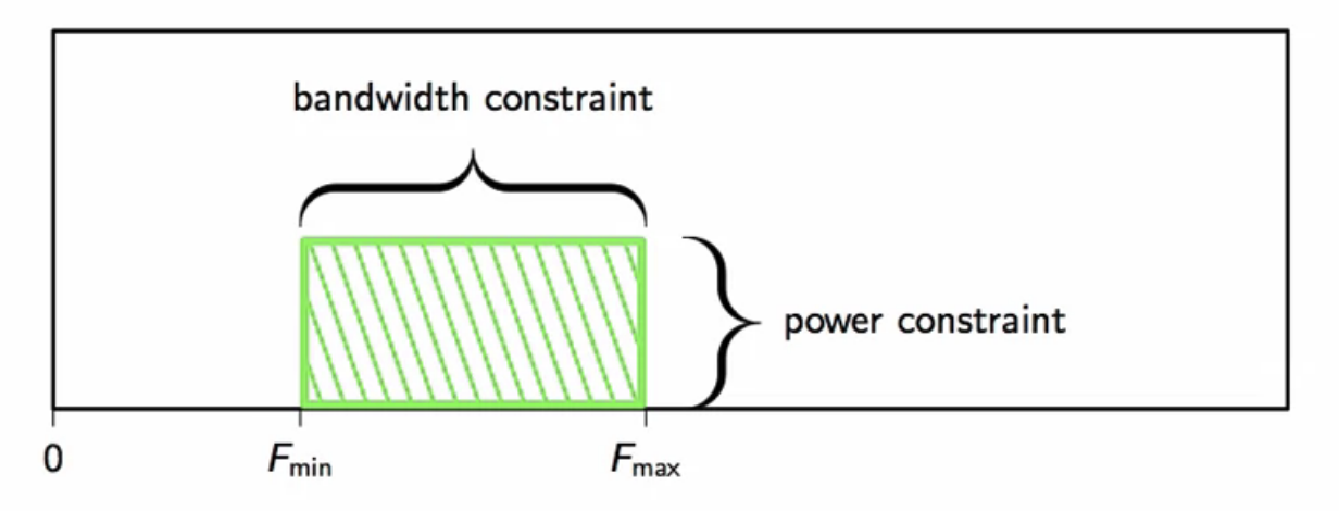
fig: channel capacity representation

bandwidth and capacity

• consider a situation where information encoded as a sequence of digital samples
  • is to be transmitted over a continuous-time channel
• the digital sequence is interpolated with an interval $T_s$
• if $T_s$ is small:
  • more information per unit time - information is dense in time
  • trade-off is the bandwidth of signal will increase
    • bandwidth is proportional to $T_s$
    • $\left|\Omega \right|>{\Omega }_N=\frac{\pi }{T_s}$

power and capacity

• all channels introduce noise
  • receiver has to guess what was transmitted
• consider integers between 1 and 10 are being transmitted
  • and noise variance is 1
  • this causes a lot of guessing errors
  • the variance is in the range of the resolution of the numbers transmitted
• transmit only odd numbers
  • less information i.e. lesser information
  • but lesser errors
  • snr is higher

channel capacity examples

AM radio channel

• input is filtered in a lowpass operation
• then a simple sinusoidal modulation is applied
• the modulated signal is sent to an antenna where it is pushed into the radio spectrum

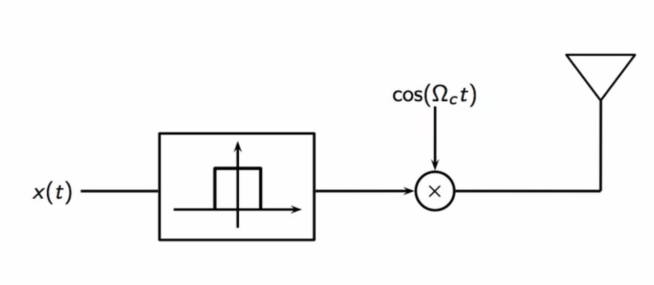
fig: AM radio channel

• the AM spectrum:
  • 530 kHz - 1.7 MHz: scarce resource
  • each AM channel in the radio spectrum is 8kHz
  • each radio station gets allocated a specific channel
• everybody has to share the radio bandwidth so the bands are regulated by law
  • specifically, power in the bandwidth is regulated
  • daytime/nighttime AM propagation behavior is very different
    • AM travels much further nights
  • too much AM power creates interference with other signals
  • too much power poses health hazards

telephone channel

• called switched telephone network
• phone connected to telephone exchange (CO - central office)
  • last mile cable
  • usually a couple km long
• routing is done based on the number dialled by the incoming calls
• exchange in the past was mechanical with rotary switches
  • now they are digital switches
• the network maybe wires, fibres, satellites links and such

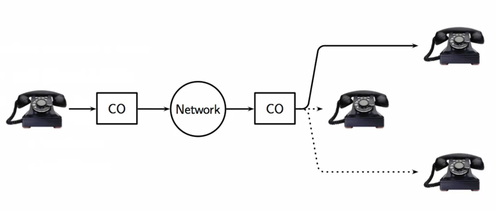
fig: AM radio channel

• the channel itself is conventionally limited to 300Hz to 3000Hz
• power limited to 0.2-0.7 ms forced by law
  • exact limit based on the hardware used
  • to protect hardware
• SNR is high: around 30dB
  • analog cables in the ground
  • not a lot of interference

---

communication system design

• everything is kept digital until signal needs transmitting through a physical channel
• all-digital paradigm
  • all signal operations are performed in the digital domain
• signal transmittance is done in physical channels
  • signal has to be modified to adhere to channel capacity
  • this is done at the transmitter
• the channel capacity challenge looks similar to filter design challenge

fig: channel capacity specs - similar to filter design specs

• the physical channel capacity is converted to digital specs
• the nyquist frequency i.e. the minimum sampling frequency is chosen based on the bandwidth

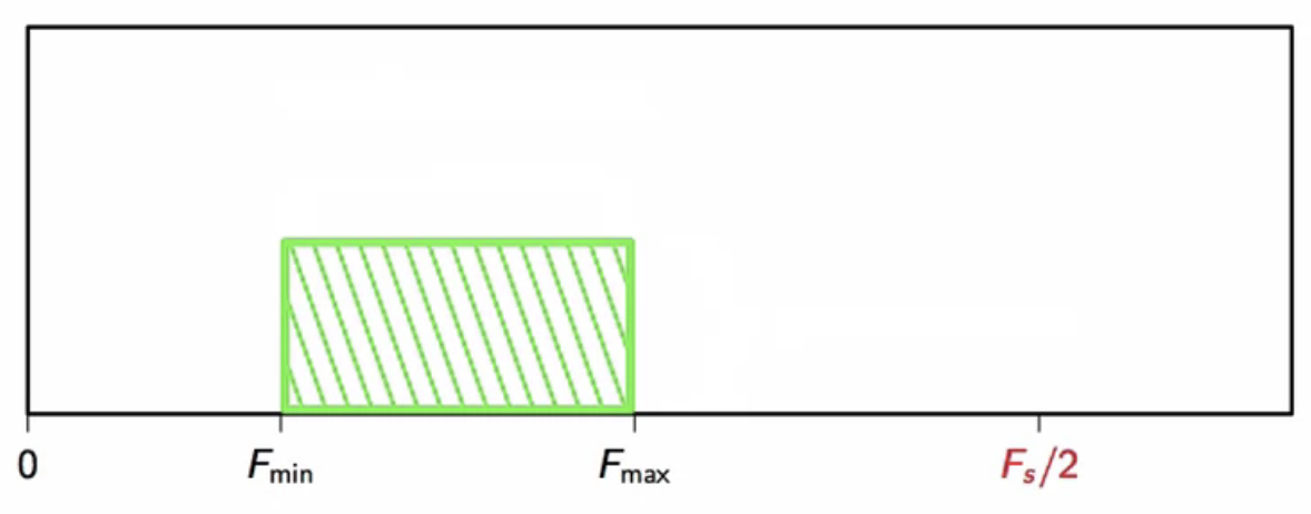
fig: selecting the sampling frequency, given channel capacity

• in the digital domain, maximum frequency is set to $\pi$ $$\Omega =2\pi \frac{F}{F_s}$$

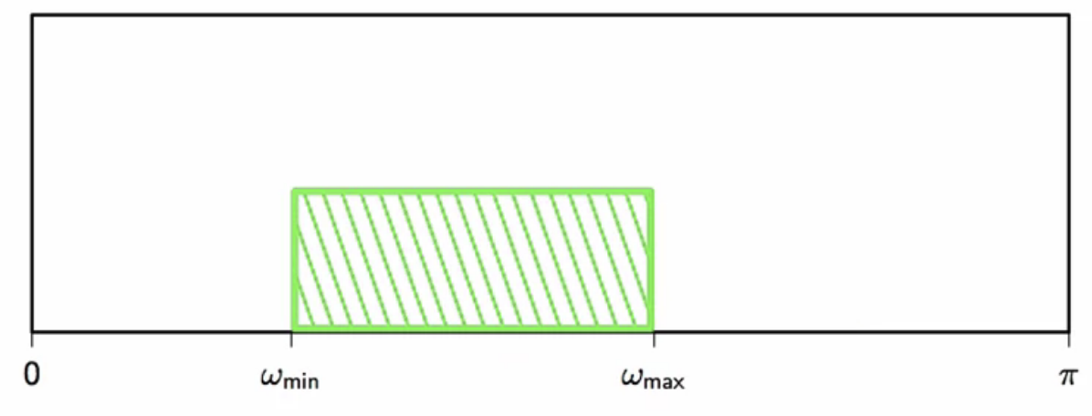
fig: converting to digital domain

transmitter design

• a set of hypothesis is adhered to when designing transmission systems

common transmitter hypothesis

• map bitstream into a sequence of symbols $a\left[n\right]$
  • using a mapper
  • eg: mapping bits to decimal value
• model $a\left[n\right]$ as a white random sequence
  • assume bitstream is completely random
  • incase of orderly sequence i.e. silence stretch in music
    • scrambler operation on bitstream ensures randomness
    • scrambling is a superficial processing tool
    • is completely invertible at receiving end
• then convert sequence $a\left[n\right]$ to a continuous-time signal
  • output must be within channel constraints

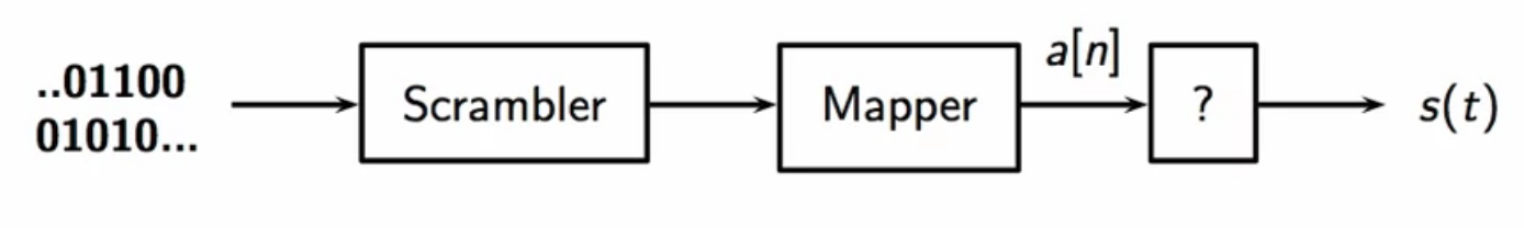
fig: transmitter design scheme

---

bandwidth control

challenge #1: bandwidth constraint

• the scrambled bitsream is random and white
• its power spectrum density is simply its variance
• so has constant power over the entire frequency spectrum
  • however the power has to fit only the frequency bandwidth of the specs of the analog channel

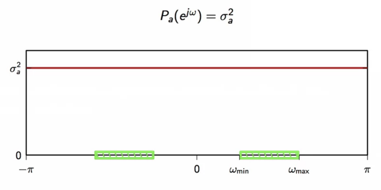
fig: distribution of power of scrambled sequence and spec bandwidth

• bandwidth constraint demands control over the support of the signal
• the full-frequency-band of the scrambled signal needs to be shrinked to the channel bandwidth

multirate techniques

• tools for bandwidth controls
• key idea of multirate technique:
  • increase or decrease the number of samples in a discrete-time signal
• equivalent to going to continuous-time and re-sampling
  • staying the digital world is cleaner
  • so the process of conversion and back-conversion is mimicked digitally

upsampling via continuous-time

• in continuous-time, upsampling scheme looks like the following

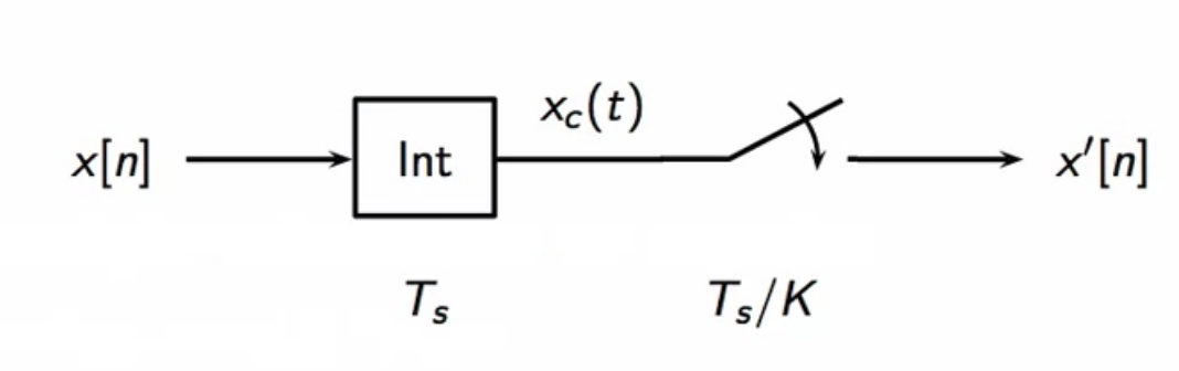
fig: interpolation and higher rate sampling - upsampling through continuous-time domain

• for $K=3$

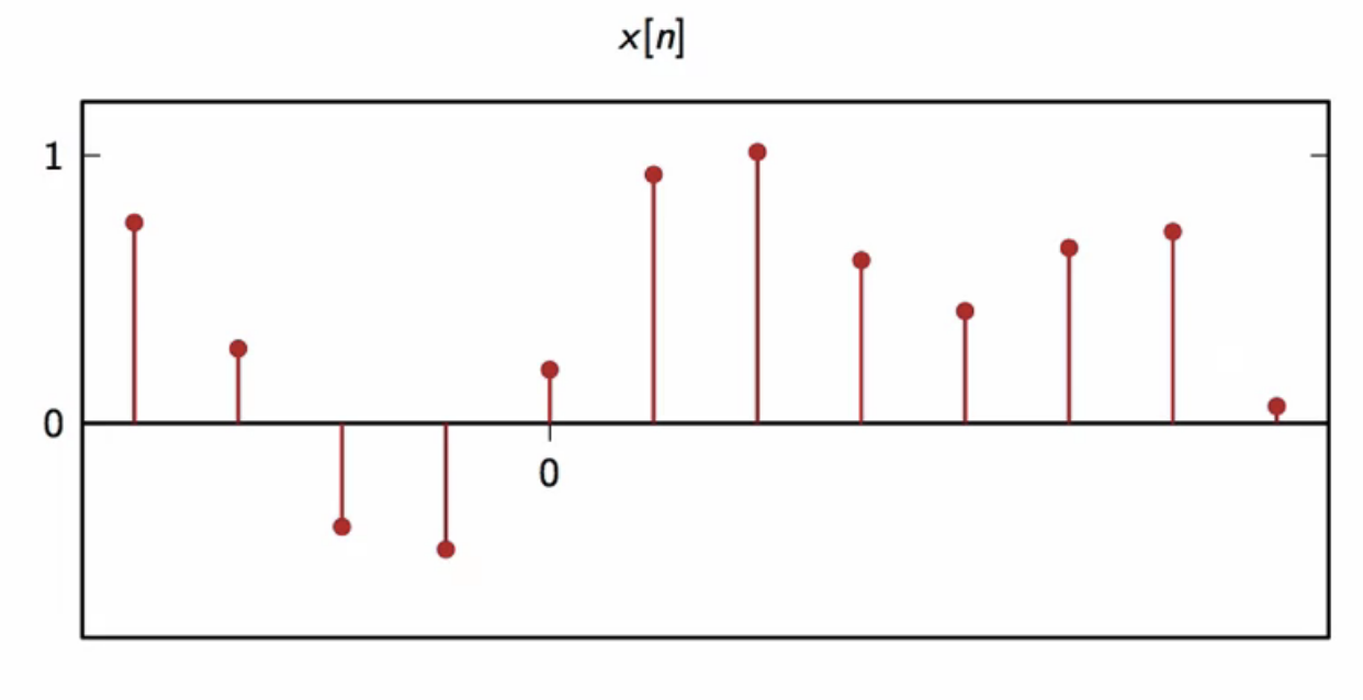
fig: consider a sequence that needs upsampling

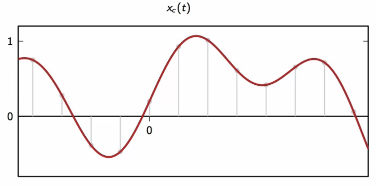
fig: interpolated sequence in continuous-time

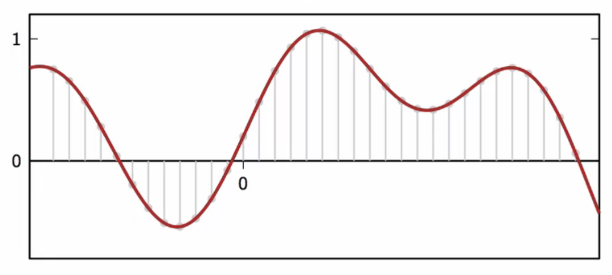
fig: 3 times higher frequency sampling

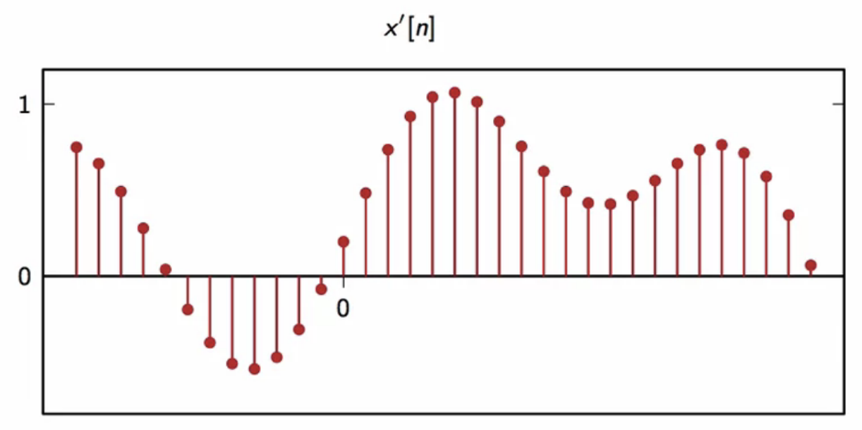
fig: resulting upsampled frequency

• choice of interpolation interval is arbitrary
• for $T_s=1$, the interpolated signal is $$x_c=\sum _{m=-\infty }^{\infty }x\left[m\right]sinc(t-m)$$

• the upsampled signal is $$\begin{array}{ccc}{x}^{\prime }& =x_c(\frac{n}{K})& =\sum _{m=-\infty }^{\infty }x\left[m\right]sinc(\frac{n}{K}-m)\end{array}$$

• in the frequency domain, the process looks like the following

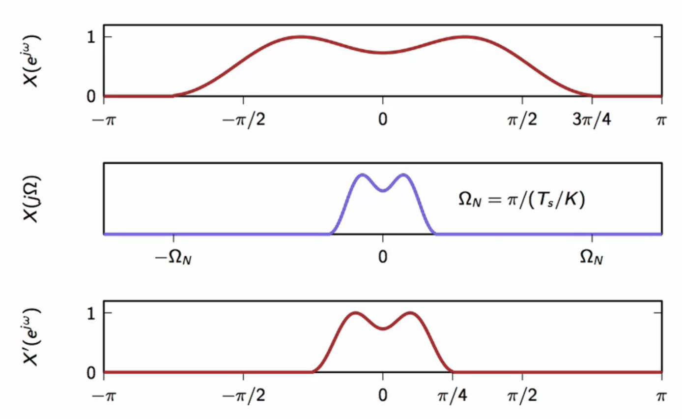
fig: spectrum of input signal (top); spectrum of interpolated signal (middle); spectrum of re-sampled i.e. upsampled signal (bottom)

• note how the upsampled signal takes up a smaller bandwidth than the signal it was upsampled from

upsampling in digital-time

• keeping in mind the all-digital paradigm, it is desired to upsample within the digital domain

• here, the number of samples needs to be increased by K
• such that $x_U\left[m\right]=x\left[n\right]$ when $m$ is multiple of $K$
  • to be able to recover original signal
• for lack of better strategy, put zeros elsewhere
  • insert $K-1$ zeros in between consecutive samples
• example: for $K=3$ $$x_U\left[m\right]=\dots x\left[0\right],0,0,x\left[1\right],0,0,x\left[2\right],0,0\dots$$

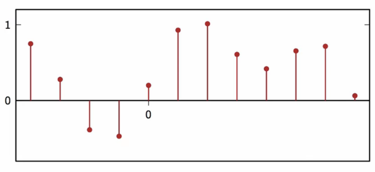
fig: sequence to be upsampled

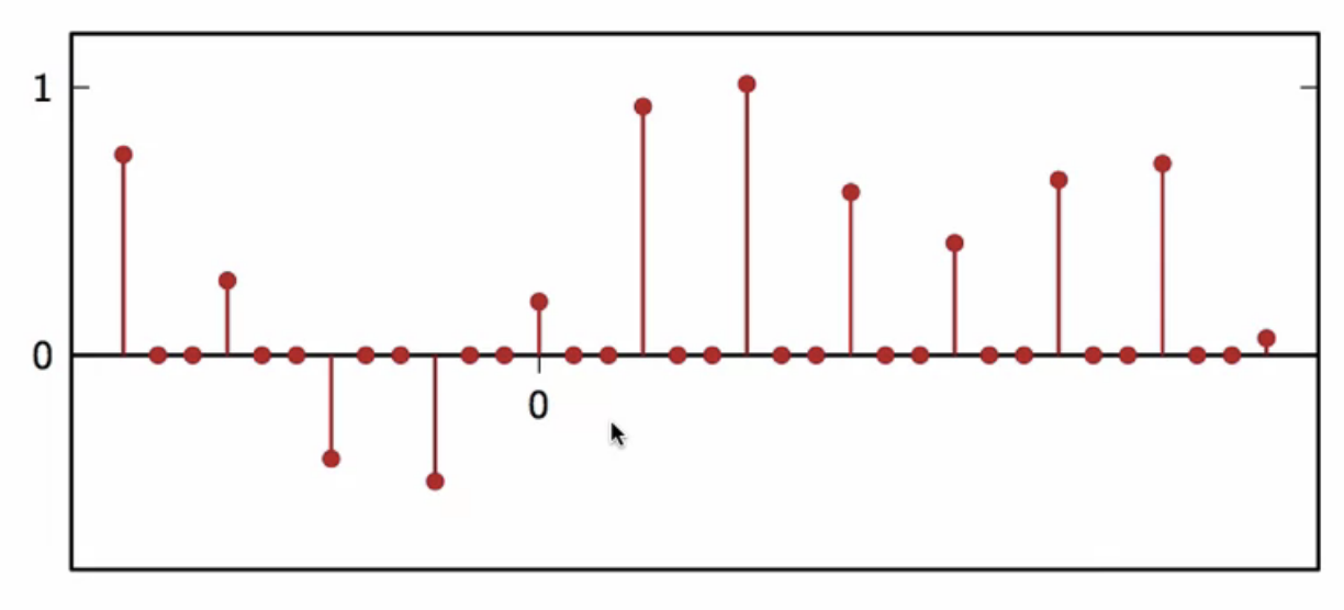
fig: upsampled signal ($K=3$)

• the fourier transform of the upsampled sequence is $$\begin{array}{cccc}{X}_U\left(e^{j\omega }\right)& =\sum _{m=-\infty }^{\infty }{x}_U\left[m\right]e^{-j\omega m}& =\sum _{n=-\infty }^{\infty }x\left[n\right]e^{-j\omega nK}& =X_U\left(e^{j\omega K}\right)\end{array}$$

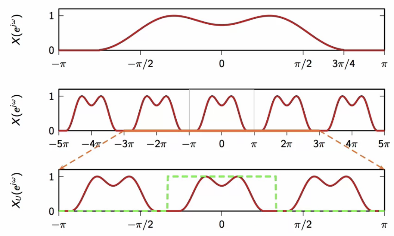
fig: spectrum of signal to be upsampled (top); periodic spectrum of signal to be upsampled (middle); spectrum of upsampled signal (bottom)

recovery with downsampling

• the resulting upsampled signal has K copies in the full $[-\pi ,\pi ]$ bandwidth spectrum
  • $K=3$ in this case
• a lowpass filter has to be applied to extract only one copy in the center
  • with a cutoff frequency $\frac{\pi }{K}$
• recovery in time domain
  • insert $K-1$ zeros after every sample
  • ideal lowpass filtering with ${\omega }_c=\frac{\pi }{K}$

$$\begin{array}{ccccc}{x}^{\prime }& =x_U\ast sinc(\frac{n}{K})& =\sum _{i=-\infty }^{\infty }{x}_U\left[i\right]sinc(\frac{n-1}{K})\text{substitute}& i=mK& =\sum _{m=-\infty }^{\infty }x\left[m\right]sinc(\frac{n}{K}-m)\end{array}$$

• downsampling is used to recover the upsampled sequence on the received side $$x\left[n\right]=x_U\left[nK\right]$$
• the filter used for lowpass has to either be ideal or fulfill the interpolation property
  • i.e. impulse response of filter should be the delta function
• downsampling of generic signals more complicated than upsampling
  • aliasing has to be dealt with as some samples are begin discarded

fitting the transmitter spectrum

• the channel imposes a frequency constraint
  • that signal frequency must only be between $F_{min}$ and $F_{max}$
  • this has to be translated to the digital domain

fig: selecting the sampling frequency, given channel capacity

• let $W=F_{max}-F_{min}$
  • difference on the bandwidth limits in the positive half of the frequency spectrum
• pick $F_s$ such that $F_s>2F_{max}$

• $F_s=KW,K\in N$

• in the digital domain,
  • ${\omega }_{max}-{\omega }_{min}=2\pi \frac{W}{F_s}=\frac{2\pi }{K}$
  • may simply be upsampled by K
  • the width obtained so will fit over the channel bandwidth
• upsampling does not change the data rate
• W symbols per seconds are produced and transmitted
• this is then upsampled by K which is equal to the sampling frequency
• W is the baud rate of the system
  • is equal to the available positive bandwidth
  • fundamental data rate of the system

fig: transmitter schematic after upsampling to fit channel bandwidth

• in the frequency spectrum this process looks as follows

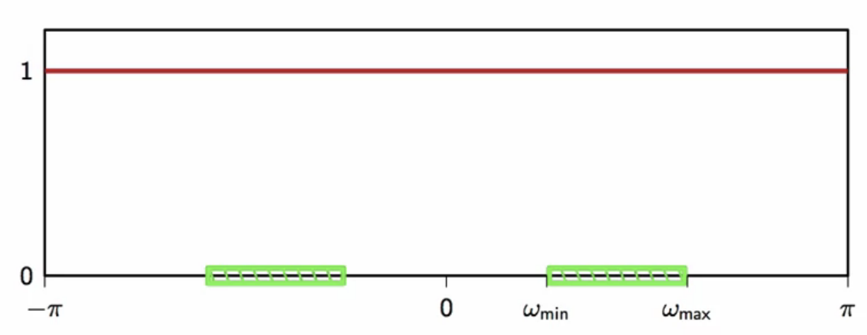
fig: scrambled white random signal

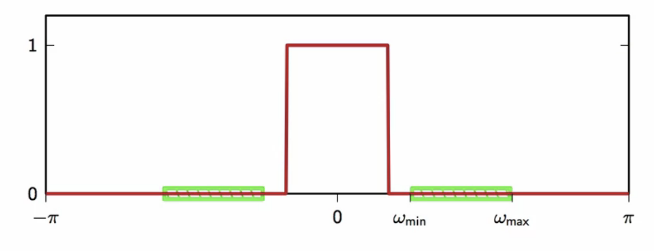
fig: upsampled lowpass filtered signal

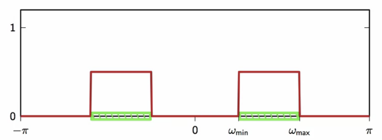
fig: modulated to fit carrier bandwidth

raised cosines

• FIR filters will be used in lowpass filtering after upsampling

• sinc lowpass filter is difficult to implement in practice

  • the raised cosine filter is used instead

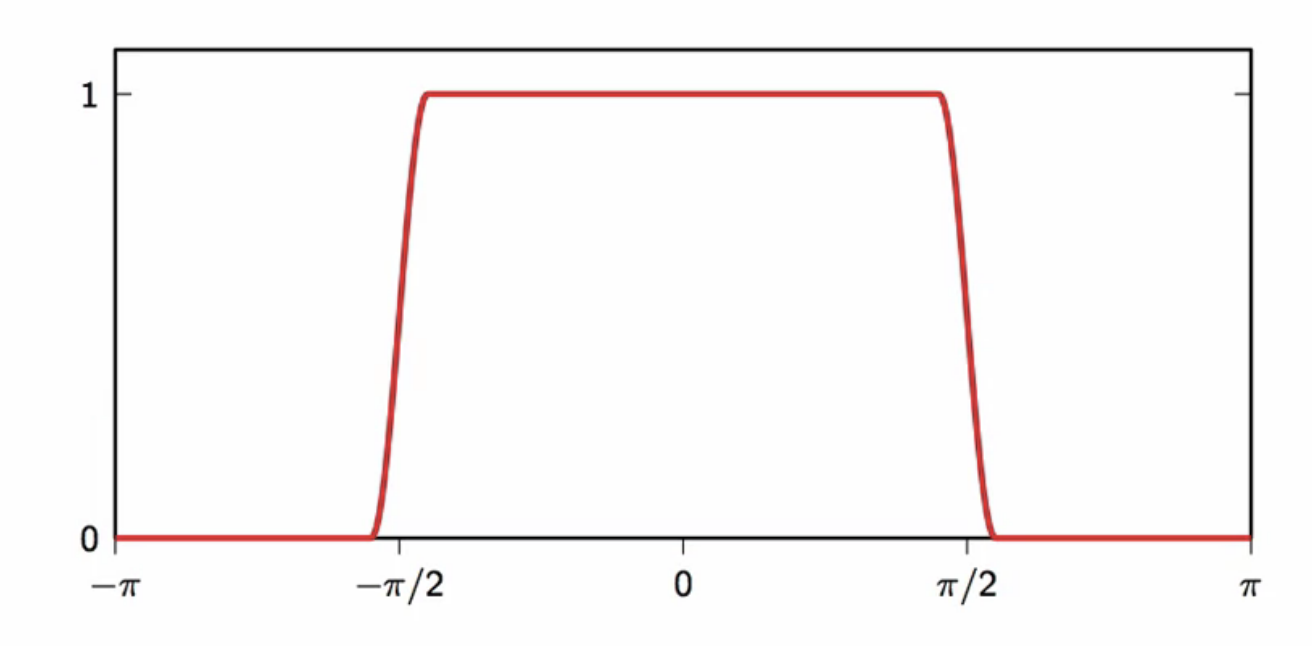
fig: raised cosine lowpass filter frequency response

• has a parameter to tune the gentleness of the transiton from passband to stopband

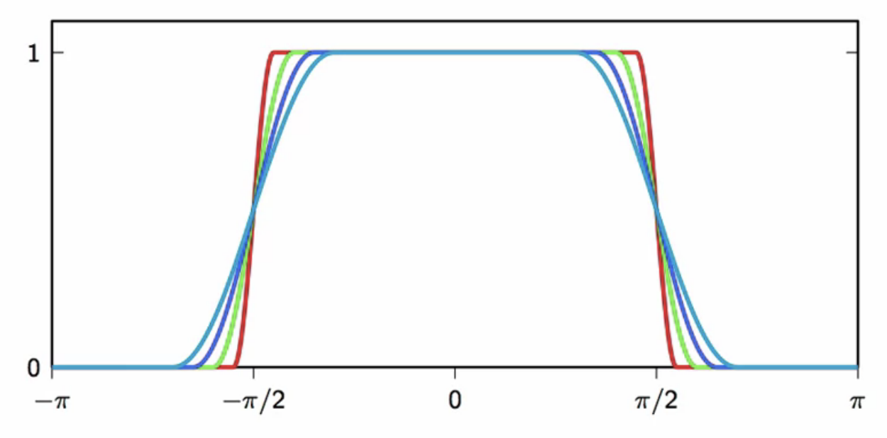
fig: gentler raised cosine filters - tunable parameter

• raised cosine filter is an ideal filter, but
  • is easier to approximate than the sinc filter
  • also satisfies the interpolation property of filters
• even short approximations can provide a good response because of the nature of its impulse response

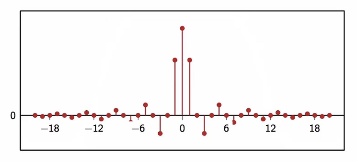
fig: impulse response of raised cosine filter

---

power control

• transmission reliability
  • transmitter sends a sequence of symbols $a\left[n\right]$
  • receiver obtains a sequence $\hat{a}\left[n\right]$
    • this is only an estimate of the transmitted signal
    • noise has leaked into the symbol
  • even if channel doesn’t distort signal, noise cannot be avoided
    • $\hat{a}\left[n\right]=a\left[n\right]+\eta \left[n\right]$
  • when noise is large
• encoding schemes
  • PAM: pulse amplitude modulation
  • QAM: quadrature amplitude modulation

probability of error

• depends on
  • power of the noise w.r.t power of signal
  • decoding strategy
  • the transmission symbols alphabet
• increasing throughput does not necessarily increase the error

transmission symbols alphabet

• a randomized bitstream is coming in
• some upsampled and interpolated samples need to be sent over the channel
• how are samples obtained from bitstream?

mapper

• splits incoming bitstream into chunks
• assign a symbol $a\left[n\right]$ from a finite alphabet $A$ to each chunk

slicers

• receives a value $\hat{a}\left[n\right]$
• decide which symbol from $A$ is closest to $\hat{a}\left[n\right]$
• piece back together the corresponding bitstream

two-level signalling

• given:
  • $G$: amplitude of signal
  • ${\sigma }_0$: standard deviation of noise
• probability of error

$$\begin{array}{cccc}{P}_{err}& =erfc(\frac{G}{{\sigma }_0})& =erfc(\frac{{\sigma }_s}{{\sigma }_0})& =erfc\left(\sqrt{SNR}\right)\end{array}$$

• probability of error decays exponentially with the signal-to-noise-ratio
• this exponential decay trend is the norm in communication systems
  • while the absolute error might change depending on the constants

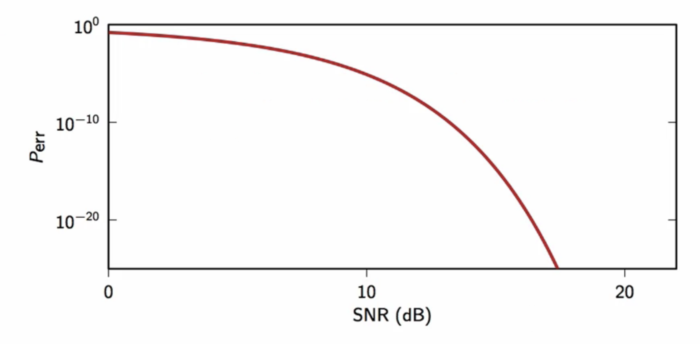
fig: two-level signalling probability error function

takeaways

• increase signal gain G (amplitude) to reduce probability of error
• increasing G increase the power
• keep in mind power cannot exceed channel constraint

pulse amplitude modulation (PAM)

• mapper
  • split incoming bitstream into chunks of $M$ bits
  • chunks define a sequence of integers $k\left[n\right]\in 0,1,\dots ,2^M-1$
  • $a\left[n\right]=G\left(\right(-2^M+1)+2k[n\left]\right)$
    • odd integers around zero
    • G: gain factor
• slicer
  • $a^{\prime }\left[n\right]=arg{min}_{a\in A}\left[\right|\hat{a}\left[n\right]-a\left|\right]$

error analysis

• result very similar to two-level signal error analysis
• bi-level signalling is PAM with M = 1

example: M = 2, G = 1

• distance between points is 2G
  • points are indicated by the diamond markers
• using odd integers creates a zero-mean sequence

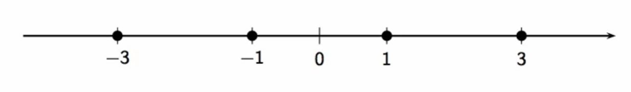
fig: pulse amplitude modulator; M = 2; G = 1

quadrature amplitude modulation (QAM)

• mapper:
  • split incoming bitstream into chunks of $M$ bits
    • $M$: even
  • use $\frac{M}{2}$ bits to define a PAM sequence $a_r\left[n\right]$
  • use the remaining $\frac{M}{2}$ bits to define an independent PAM sequence $a_i\left[n\right]$
  • $a\left[n\right]=G\left(a_r\right[n{]}_j{a}_i\left[n\right])$
  • so the resulting
• slicer:
  • $a^{\prime }=argmi{n}_{a\in A}\left[\right|\hat{a}\left[n\right]-a\left|\right]$

example: M = 2, G = 1

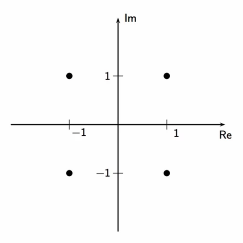
fig: quadrature amplitude modulator; M = 2; G = 1

example: M = 4, G = 1

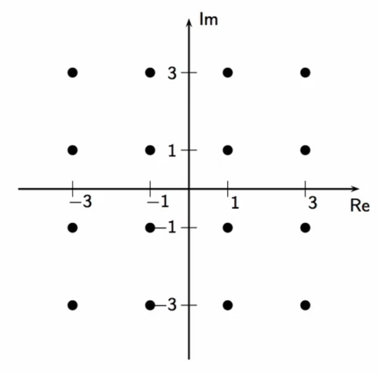
fig: quadrature amplitude modulator; M = 4; G = 1

example: M = 8, G = 1

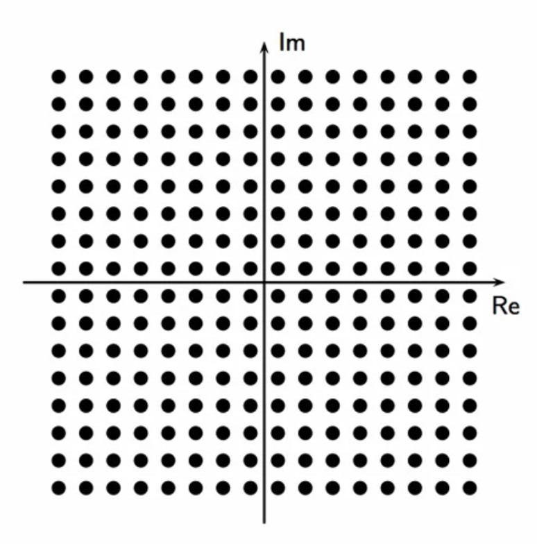
fig: quadrature amplitude modulator; M = 8; G = 1

probability of error

• the slicer adds the square area centered around the symbol

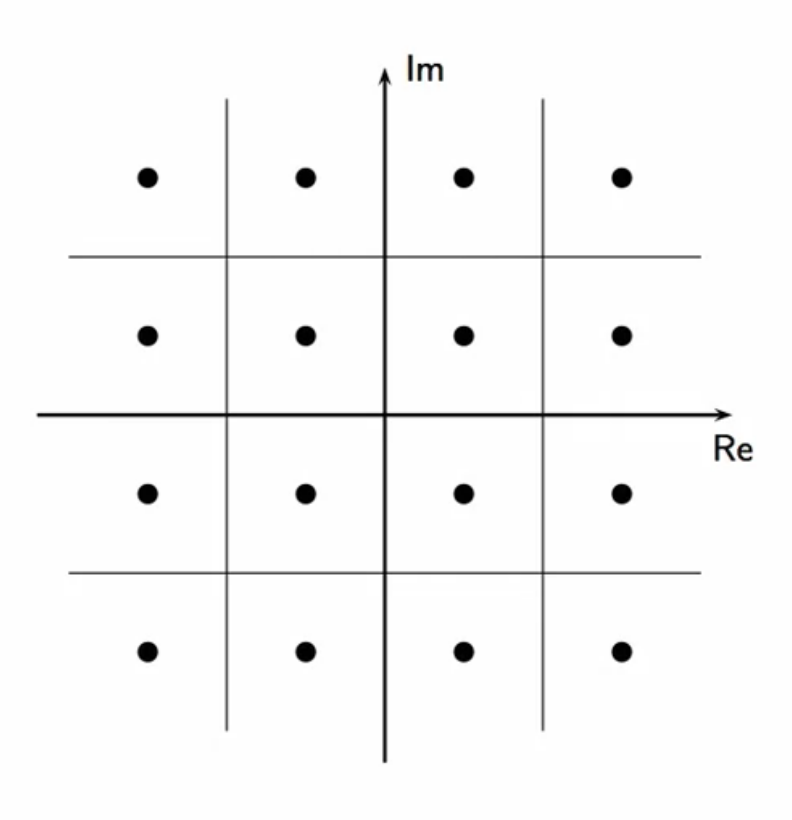
fig: quadrature amplitude modulator - error analysis

• each received symbol $\hat{a}$ is the sum of the original sample and an error $\hat{a}\left[n\right]=a\left[n\right]+\eta \left[n\right]$
• the error term $\eta \left[n\right]$ is assumed to be
  • a complex value
  • with gaussian distribution of equal variance
  • in both real and complex components

• the probability of error is given by $$\begin{array}{cccc}{P}_{err}& =P\left[\right|Re\left(\eta \right[n\left]\right)|>G]+P\left[\right|Im\left(\eta \right[n\left]\right)|>G]& =1-P\left[\right|Re\left(\eta \right[n\left]\right)|<G\wedge |Im\left(\eta \right[n\left]\right)|<G]& =1-{\int }_D{f}_{\eta }\left(z\right)dz\end{array}$$

• so now the slicer area is converted to a circle from being a square

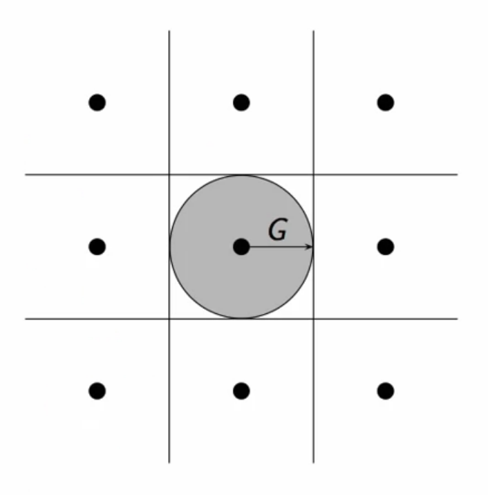
fig: quadrature amplitude modulator - error analysis

• if noise variance is assumed to be $\frac{{\sigma }_0^2}{2}$
  • in both real and imaginary component

• probability of error is approximated by $$P_{err}\approx {\exp }^{\frac{-G^2}{{\sigma }_0^2}}$$

• to obtain probability of error as a function of SNR:
  • compute power of signal

• assume all symbols equiprobable and independent, variance of signal is $$\begin{array}{ccc}{\sigma }_s^2& =G^2\frac{1}{2^M}\sum _{a\in A}|a{|}^2& =G^2\frac{2}{3}(2^M-1)\end{array}$$

• plugging this back into the equation of error probability $$P_{err}\approx {\exp }^{\frac{-G^2}{{\sigma }_0^2}}\approx {\exp }^{-3\ast SNR\ast 2^{(M+1)}}$$

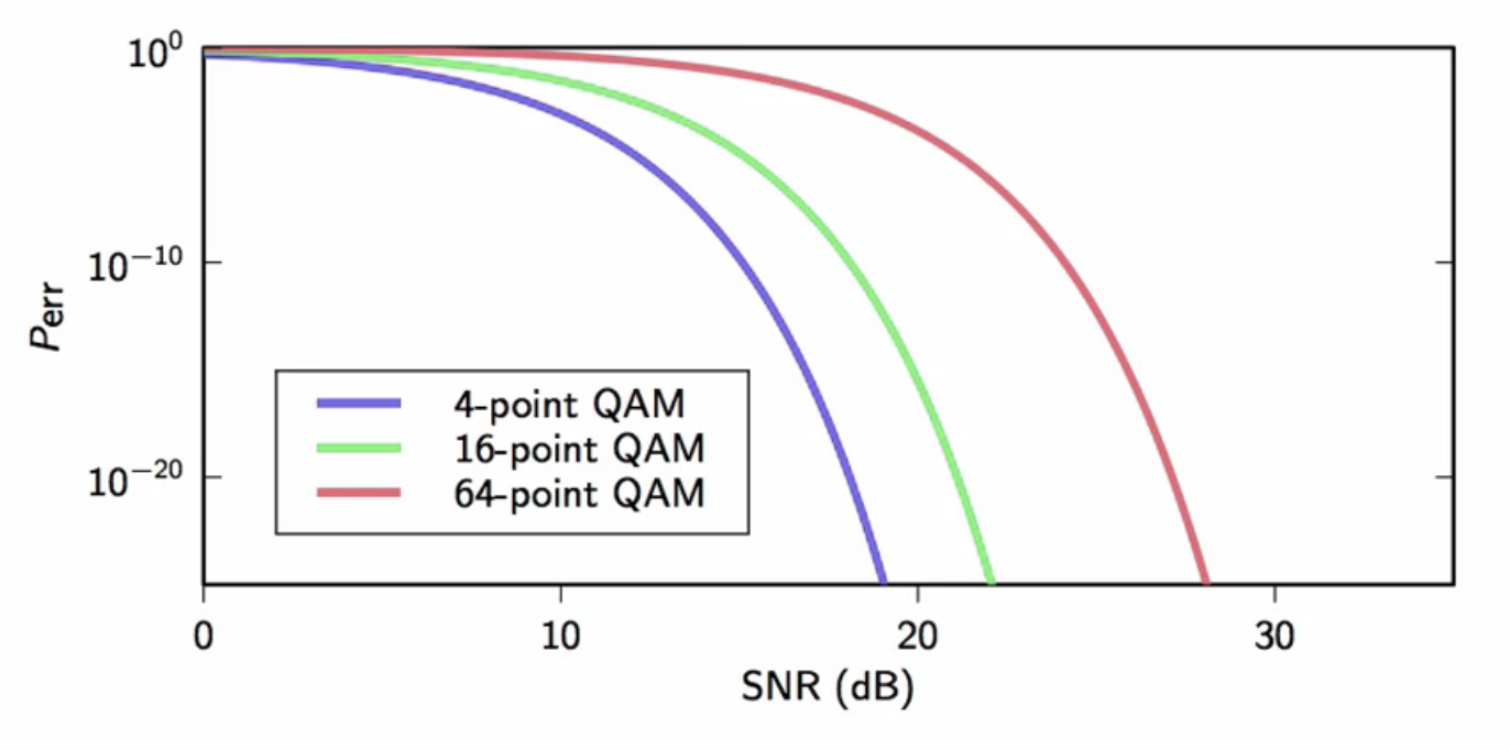
fig: plotting error probability on a log-log scale

• probability of error increases with number of points, because the area associated with each point becomes smaller
  • the decision at the receiving end in classifying a received sample to a symbol become harder
  • because it could belong to more other symbols than when the number of symbols is less

QAM design procedure

• pick a probability of error that is acceptable (i.e. ${10}^{-6}$)
• find out the SNR imposed by the channel’s power constraint
• find $M$ using $M=lo{g}_2(1-\frac{3}{2}\frac{SNR}{\ln \left(p_e\right)})$
  • size of symbol constellation
  • might need rounding
    • to even number
• final throughput (data rate) will be $MW$
  • M: size of symbol constellation
  • W: baud rate

regroup-1

• bandwidth constraint fit discussed
• given power constraint, the bits/symbol can be calculated
• we know the theoretical throughput of the transmitter
• how to transmit complex symbols over a real channel?

---

references

• moore’s law