[DSP] W08 - Receiver Design
contents
- signal picks up noise while propagating in the channel
- it also get distorted as the channel acts as some sort of filter,
- that is not necessary lowpass or linear-phase
- interference occurs as well
-
there might be parts of the channel that might assumed to be usable and actually not
- the receiver has to deal with a copy of the transmitted signal
- very far from the idealized version used in the math for designing the transmitter
- adaptive filtering techniques enable digital receivers to cope with the distortions and the noise introduced by the channel
- topics: advanced signal processing classes
- this is an overview
- your ADSL receiver for instance
- allows high data rates
receiver design
- following is the sound made by a dial-up internet modem
- when connecting to the internet
- for graphical analysis of this sound, refer to receiver schematic below
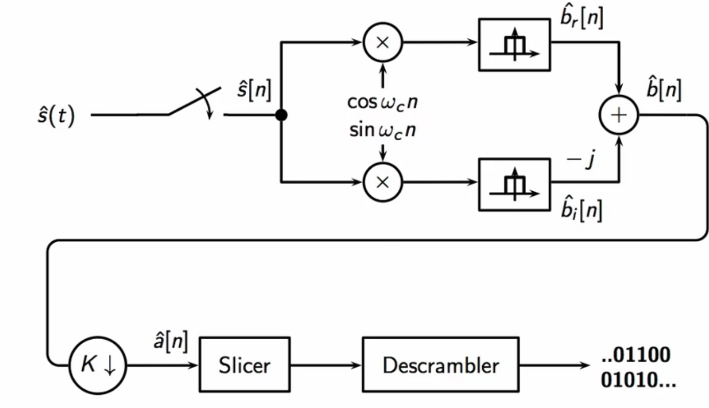
fig: QAM receiver signal flow schematic
- baseband complex samples \( \hat{b}[n] \) are plotted on the complex plane
- if the input at the receiver is a signal \( \hat{s}[n] = \cos(( \omega_c + \omega_0 ) n ) \)
- the obtained baseband for this is \( \hat{b}[n] = e^{j\omega_0 n} \)
- so they point on the unit circle on the argand plane
- the angle between successive points will be \( \omega_0 \)
pilot tones
- the receiver sends pilot tones
- pilot tones are simple sinusoids used to probe the channel
- channel probing
-
used to gauge the response at particular frequencies
- some components
- many sinusoids
- which have abrupt phase changes
- phase reversals are used as time markers
- to estimate propagation delay of channel
- training sequence
- known sequence is sent my transmitter
- the receiver uses channel response to this known sequence to train an equalizer to offset channel effects
- handshake procedure between transmitter and receiver
- just before core information transmission begins
- low bitrate QAM transmission using only four points
- 2 bits per symbol
- parameters exchange of speed, constellation size etc
- since only 4 points constellation,
- so even in noisy conditions ensure vital information exchange
- data transmission proper
- many sinusoids
receiver function
- challenges faced at the receiver and measures taken to offset each challenge
- interference
- handshake and line probing
- propagation delay
- delay estimation
- linear distortion
- adaptive equalization
- clock drifts between the receiver and the transmitter
- timing recovery
- advanced topic
- interference
main challenges
- challenge distortion
-
time-varying discrepancies in clocks \( T_s^{\prime} = T_s \)
- the channel is approximated as a linear filter in the continuous-time domain to begin analysis
- \( D(j\omega) \): filter response
- the filter is assumed to introduce all distortion and delays
- signal at receiver end: \( \hat{s}(t) \)
- delayed and distorted version of transmitted signal
- clock of transmitter: \( T_s \)
- clock of receiver: \( T_s^{\prime} \)
- no guarantee these two are synchronized
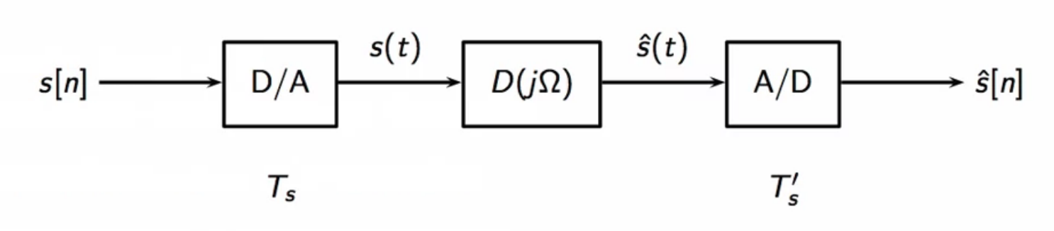
fig: DAC at transmitter and ADC at the receiver
delay compensation
- assuming the following are in sync
- clock of transmitter: \( T_s \)
- clock of receiver: \( T_s^{\prime} \)
- channel introduces a delay of \(d\) seconds
- channel is a simple delay block
- \( \hat{s}(t)=s(t-d) \rightarrow D(j\Omega) = e^{-j\Omega d} \)
- we can write \( d = (b + \tau) T_s \) with \( b \in \mathbb{N} \) and \( \vert \tau \vert < \frac{1}{2} \)
- \(b\) is the bulk delay
-
\(\tau\) is the fractional delay
- bulk delay is simple to tackle
- also called the integer delay
- they are simply the delay that the channel adds to the signal
- this does not sift the peaks of the data with respect to the sampling interval
- discontinuities in pilot tones help figure out bulk delay
- impulses cannot be used as they are full band and get filtered out
- the fractional delay is more involved
- it shifts the peaks with respect to the sampling intervals
- interpolation is used to get the fractional delay compensation
- transmit \( b[n] = e^{j\omega_0 n} \)
- \( s[n] = \cos((\omega_c + \omega_)) n ) \)
- receive \( \hat{s}[n] = \cos((\omega_c + \omega_0) (n - b - \tau)) \)
- after demodulation and bulk delay offset
- \( \hat{b}[n] = e^{j\omega_0(n-\tau)} \)
- multiply by known frequency
- \( \hat{b}[n]e^{-j\omega_0 n} = e^{-j \omega_0 \tau} \)
- after offsetting bulk delay
- \( \hat{s}[n] = s(n-\tau) T_s \)
- subsample values need to be computed
- in theory, compensate with a sinc fractional delay
- \( h[n] = sinc(n=\tau) \)
- in practice use lagrange approximation
- practical application of lagrange polynomials
- lagrange approximation is around \( n \)
- to compute \(x(n + \tau) \) with \( \vert \tau \vert < \frac{1}{2} \)
\[ \begin{align}
x_L(n;t) & = \sum_{k = - N}^{N} x[n-k] L_k^{(N)} (t) \
L_k^{(N)} (t) & = \prod_{i = -N; i \neq k}^{n} \frac{t-i}{k-i} \
\text{ where } & = k = -N, \ldots , N \
\end{align}
\]
- \( x(n+\tau) \approx x_L(n;\tau) \)
- so, in summary
- estimate the delay \(\tau\)
- compute the \( 2N + 1 \) lagrangian coefficients
- filter with the resulting FIR
adaptive equalization
- measure to compensate for distortion
- let the channel distortion be \( D(z) \)
- \( E(z) \) is the equalizer compensation to offset channel distortion
- in theory \( E(z) = 1/D(z) \)
- but \(D(z)\) is not known
-
\( D(z) \) may change over time during transmission
- hence the equalization \(E(z\) needs to adapt continuously
- following is the schematic of an adaptive equalizer
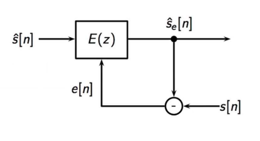
fig: core adaptive equalizer schematic
- the filter coefficient changes in time based on the error
- obtained from the output with the transmitted signal
- the exact signal is sent by the transmitter
- the receiver has the same copy to get the adaptive equalizer started
- this is a bootstrapping technique
- there are some symbols that are common to both the transmitter and receiver together
- this is called a training sequence
- handshake 4 point QAM
- the equalizer is initialized with this shared symbol set
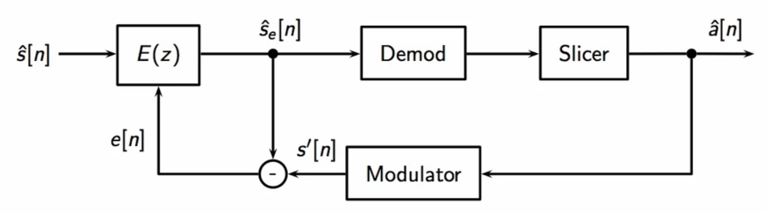
fig: adaptive equalizer schematic in the big picture
- this process of bootstrapping is not error free
- but a generally good place to get started
- details of adaptive signal processing is an advanced topic
- needs more research, reading and understanding
adsl
- ADSL: asymmetric digital subscriber line
- adsl receives signals on a copper wire channel
- DSLAM: digital subscriber line access multiplier
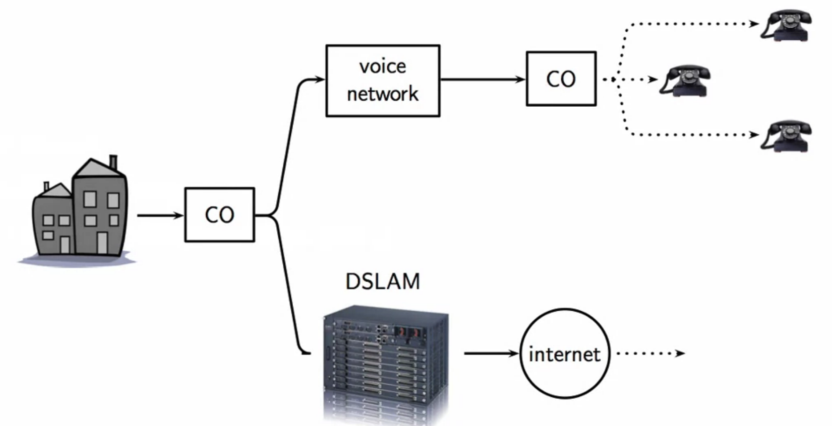
fig: telephone network overview
- last mile: copper wire connecting the home modem to the exchange (CO - central office)
- copper wire has a large bandwidth
- POTS: plain old telephone system
- the (A)symmetry in the bandwidth is the A of the ADSL
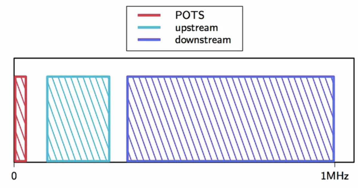
fig: adsl channel - copper wire bandwidth
channel propagation challenges
- attenuation: the uneven curve across the bandwidth
- physical wire imperfections
- parasitic capacitance
- electrical interference: large grey blog in a specific frequency region
- running the vacuum for instance raises the noise floor of the copper channel
- localized radio interference: the impulse at a specific frequency
- ship-to-shore communications: 0 - 100 kHz
- airplane communications: 100 - 500 kHz
- AM radio band: 500 kHz +
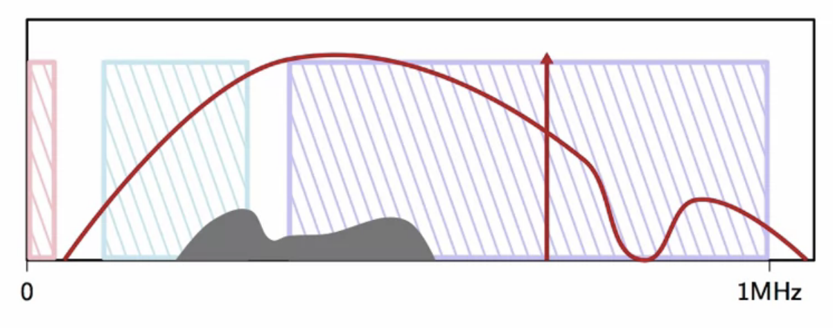
fig: adsl channel propagation challenges
- the channel is divided into independent sub-channels
- different channels are treated separately
- localized treatment in the receiver across all bands
- the cleanest channels are used to send maximum data
subchannel structure
- allocate N sub-channels over the total positive bandwidth
- equal sub-channel bandwidth \( \frac{F_{max}}{N} \)
- equally spaced sub-channels with center frequency \( \frac{kF_{max}}{N} \)
- \( k = 0, \ldots, N - 1 \)
digital design
- pick \(F_s = 2 F_{max} \)
- \( F_{max} \) is high now
- center frequency for each subchannel
- \( \omega_k - 2\pi \frac{kF_{max}/N}{F_s} = \frac{2\pi}{2N}k \)
- bandwidth of each sub-channel \( \frac{2\pi}{2N} \)
- to send symbols over a subchannel
- upsampling factor \( K \geq 2N \)
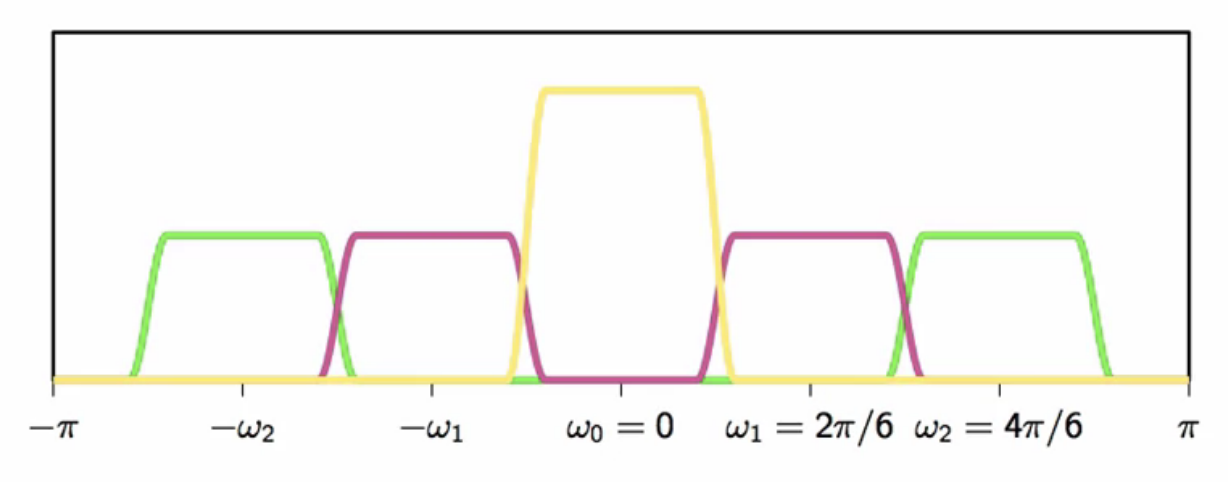
fig: subchannels of the adsl channel (N = 3)
- QAM modem is added on each channel
- decide on constellation size independently for each channel
- clean channel gets high numbered constellation
- noisy channel gets low numbered constellation
- noisy or forbidden sub-channels send zeros
- the structure of the communication scheme is sent to the receiver from the transmitter
- part of handshake procedure
- classic modulation scheme is applied in each channel as per below schematic
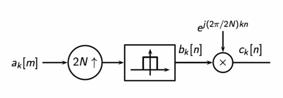
fig: modem on each sub-channel
- the receiver modem bank has several modems in parallel
- each channel has two unique attributes
- frequency of modulation
- mappers symbols series
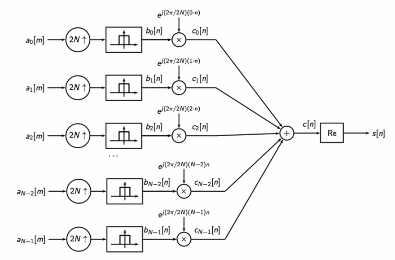
fig: modem bank
discrete multitone modulation
- the modem banks maybe seen as oscillators whose output is summed to obtain a signal
- each oscillator is scaled with an amplitude
- and phase offset
- this bank is run for N samples to get the signal
- these are constant through the generation
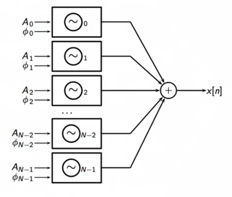
fig: oscillator bank paradigm for modem bank
- in the modem scenario, the amplitude and phase change at every sample
- they embed the complex symbol sequence
- with the discrete multitone modulation, adsl may be implemented with a simple inverse FFT
- provided that the symbols can be help constant during the whole upsampling event
- the modem structure can be mapped to the inverse DFT structure if this is done
- the ADSL trick:
- instead of using a god lowpass filter use a the 2N-tap interval indicator
\[ h[n] = \Bigg( \begin{matrix} 1 & \text{ for } 0 \leq n \leq 2N \\ 0 & \text{ otherwise } \end{matrix} \Bigg) \
\]
- instead of using a god lowpass filter use a the 2N-tap interval indicator
\[ h[n] = \Bigg( \begin{matrix} 1 & \text{ for } 0 \leq n \leq 2N \\ 0 & \text{ otherwise } \end{matrix} \Bigg) \
fig: modem on each sub-channel
- oscillator in the modulator runs freely
- with simplification, in each chunk of 2N samples, the symbol is kept constant
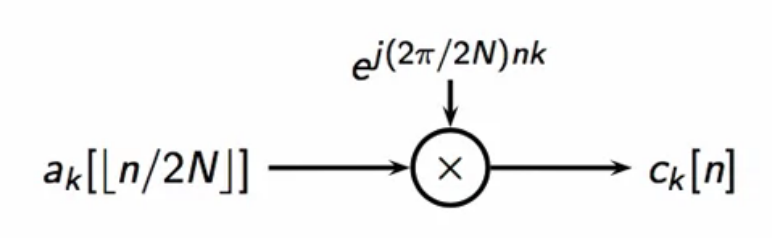
fig: simplification of subchannel modem
- aggregate bandpass signal is calculated by
\[ \begin{align}
c[n] & = \sum_{k = 0 }^{N-1} a_k[ \lfloor \frac{n}{2N} \rfloor] e^{j \frac{2\pi}{2N} nk} \
& = 2N * IDFT_{2N} \{ [ a_0[m] \text{ } a_1[m] \text{ } \ldots a_{N-1}[m] 0 \text{ } 0 \text{ } \ldots ] \} [n] \
m & = \lfloor \frac{n}{2N} \rfloor \
\end{align} \]
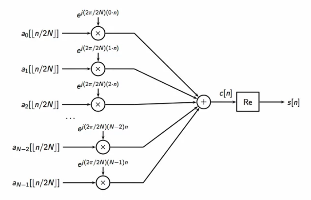
fig: simplified subchannels’ modem bank
- final goal: calculate \(s[n]\) \[ s[n] = Re\{ c[n] \} = \frac{( c[n] + c^*[n] )}{2} \]
\[ IDFT \{ [ x_0 \text{ } x_1 \text{ } \ldots \text{ } x_{N-2} \text{ } x_{N-2} ] \}^* = IDFT \{ [ x_0 \text{ } x_1 \text{ } \ldots \text{ } x_{N-2} \text{ } x_{N-2} ]^* \} \]
\[ c[n] = 2N * IDFT\{ [ a_0[m] \text{ } a_1[m] \text{ } \ldots \text{ } a_{N-1}[m] \text{ } 0 \text{ } 0 \ldots 0 ] \} [n] \]
- hence, since baseband always has read valued symbols
\[ s[n] = N * IDFT\{ [ 2a_0[m] \text{ } a_1[m] \text{ } \ldots \text{ } a_{N-1}[m] \text{ } a_{N-1}^* [m] \text{ } a_{N-2}^* [m] \ldots a_{1}^* [m] ] \} [n] \]
ADSL schematic
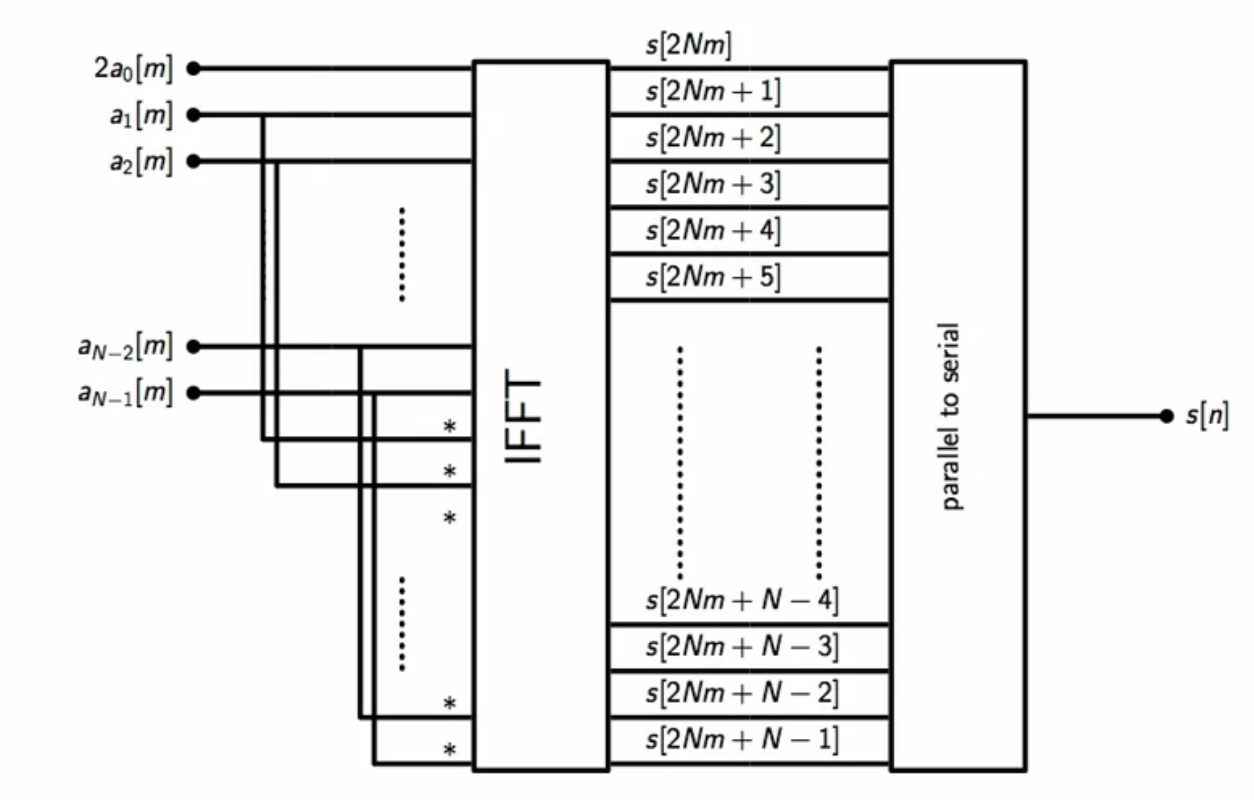
fig: simplified subchannels’ modem bank
ADSL specs
- \(F_{max} = 1104 kHz\)
- N = 256
- each QAM can send 0 - 15 bit per symbol
- forbidden channels 0 to 7
- dedicated to voice
- channels 7 - 31: upstream data
- max theoretical throughput: 14.9 Mbps (downstream)